Note
Training at Digital Earth Africa has moved! Register at learn.digitalearthafrica.org to enrol in the revised and updated 6-week training course, now called Intro to Sandbox (EN) and Introduction à la sandbox (FR). Find out more about the move on our blog.
Quiz links are no longer available from this website. Please complete the Intro to Sandbox course on learn.digitalearthafrica.org to receive a certificate.
La formation à Digital Earth Africa a déménagé ! Connectez-vous sur learn.digitalearthafrica.org pour vous inscrire à la formation révisée et mise à jour, désormais appelée Icntroduction à la sandbox (FR) et Intro to Sandbox (EN). En savoir plus sur le déménagement en consultant notre blog.
Les liens de quiz ne sont plus disponibles sur ce site Web. Veuillez suivre le cours Introduction à la sandbox sur learn.digitalearthafrica.org pour recevoir un certificat.
Import external datasets
The Digital Earth Africa Sandbox allows users to add external data such as shapefiles and .geojson files to their algorithms.
This tutorial will take you through:
The packages to import
Setting the path for the vector file
Loading the external dataset
Displaying the dataset on a basemap
Loading the satellite imagery by using the extent of the external dataset
Mask the area of interest from the satellite imagery using the extenal dataset
For this tutorial, the example external dataset is in a shapefile format.
Note
Before you proceed, ensure you have completed all lessons in the DE Africa Six-Week Training Course.
Set up notebook
In your Training folder, create a new Python 3 notebook. Name it external_dataset.ipynb. For more instructions on creating a new notebook, see the instructions from Session 2.
Load packages and functions
In the first cell, type the following code and then run the cell to import necessary Python dependencies.
import sys
import datacube
import numpy as np
import pandas as pd
import geopandas as gpd

from datacube.utils import geometry

sys.path.append('../Scripts')
from deafrica_datahandling import load_ard, mostcommon_crs
from deafrica_plotting import map_shapefile, rgb
from deafrica_spatialtools import xr_rasterize
Take note of the packages below on how they were imported with other packages above.
These packages are the packages you will need when you want to use external dataset.
import geopandas as gpd
from datacube.utils import geometry
from deafrica_plotting import map_shapefile
from deafrica_spatialtools import xr_rasterize
Connect to the datacube
Enter the following code and run the cell to create our dc object, which provides access to the datacube.
dc = datacube.Datacube(app='import_dataset')
Create a folder called data in the Training directory. Download this zip file and extract on your local machine. Upload the reserve shapefile (cpg, dbf, shp, shx) into the data folder.
Create a variable called shapefile_path,to store the path of the shapefile as shown below.
shapefile_path = "data/reserve.shp"
Read the shapefile into a GeoDataFrame using the gpd.read_file function.
gdf = gpd.read_file(shapefile_path)
Convert all of the shapes into a datacube geometry using geometry.Geometry
geom = geometry.Geometry(gdf.unary_union, gdf.crs)
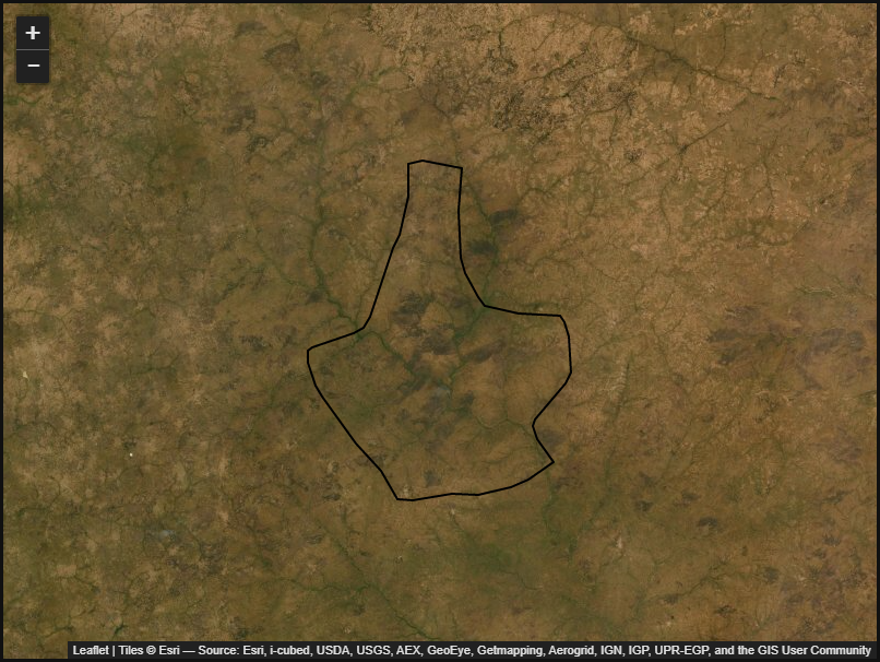
Use the map_shapefile function to display the shapefile on a basemap.
map_shapefile(gdf, attribute=gdf.columns[0], fillOpacity=0, weight=2)
Create a query object
We will replace x and y with geopolygon, as shown below. We remove the x, y arguments and replace it with geopolygon.
query = {
    'x' : x,
    'y' : y,
    'group_by': 'solar_day',
    'time' : ('2019-01-15'),
     'resolution': (-10, 10),
}
Remove x, y from query and update with geopolygon:
query = {
    'geopolygon' : geom,
    'group_by': 'solar_day',
    'time' : ('2019-01-15'),
     'resolution': (-10, 10),
}
We then identify the most common projection system in the input query, and load the dataset ds.
output_crs = mostcommon_crs(dc=dc, product='s2_l2a', query=query)

ds = load_ard(dc=dc,
              products=['s2_l2a],
              output_crs=output_crs,
              measurements=["red","green","blue"],
              **query
             )
Print the ds result.
ds
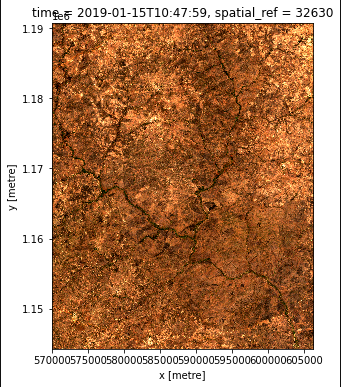
Ploting of the result
We will dipslay the returned dataset using the rgb functions.
rgb(ds)
Rasterise the shapefile
Before we can apply the shapefile data as a mask, we need to convert the shapefile to a raster using the xr_rasterize function.
mask = xr_rasterize(gdf, ds)
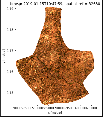
Mask the dataset
Mask the dataset using the ds.where and mask to set pixels outside the polygon to NaN.
ds = ds.where(mask)
Plot the masked result of the dataset
rgb(ds)
Conclusion
You can apply this method to already exisiting notebooks you are working with. It is useful for selecting specific areas of interest, and for transferring information between the Sandbox and GIS platorms.