Loading data in the Sandbox

Overview

In this exercise, we will load data from the datacube. First, we will set up a new notebook to work in. Then, we will load Landsat 8 data for a specific time, and use that data to plot a colour image. Finally, we will show you how to modify the load process to load and plot Sentinel-2 data.

Make a new notebook

Let’s create a new, blank Jupyter notebook for this exercise.

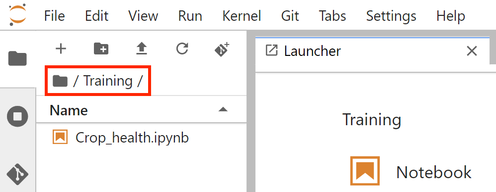
1. Navigate to the Training folder. The Training folder was created as part of Session 1, for copying and running the Crop Health notebook. If you do not have this folder in the Sandbox, you can create it by following the steps in Running a Notebook.

   

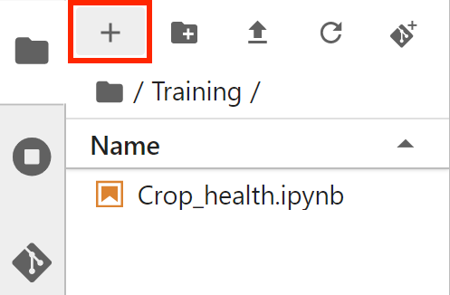
2. If Launcher is not the active tab in the main work area (right pane), click the + button at the top of the left sidebar to open the launcher in the right pane.

   

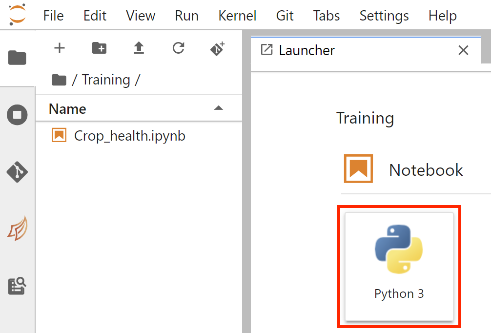
3. In the Notebook section of Launcher, select the Python 3 option to create a new notebook in the current directory.

   

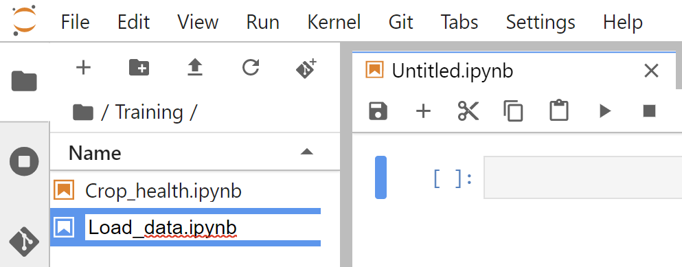
4. The new notebook will be called Untitled.ipynb, but you can rename it. Right-click the notebook in the file menu and select Rename.

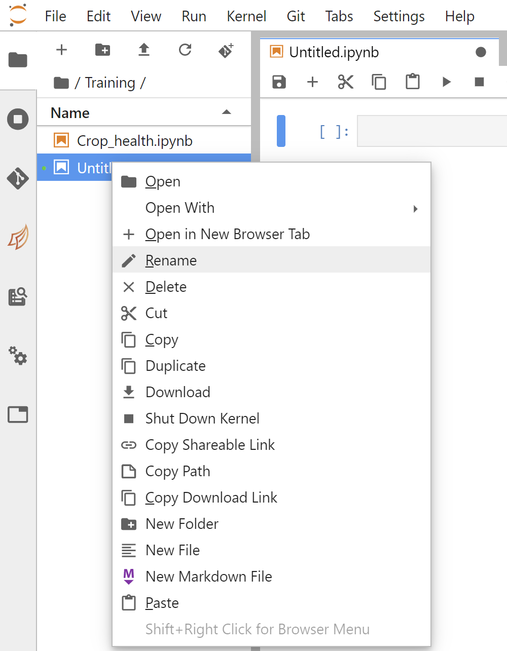
Type in the desired name. For example, we can call it Load_data.ipynb.

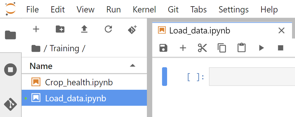
Press the Enter key to finish renaming the notebook.

Set up notebook

Load packages and functions

Packages and functions act as the toolbox of Python programming. We will import the ones which will be useful to us.

In the first cell, type the following code and then run the cell.

Note

Run a cell by pressing Shift + Enter on your keyboard.

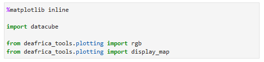
• %matplotlib inline allows us to plot graphs and maps

• The package datacube is imported to allow us to create an object that can retrieve data from the datacube, which we will do in the next cell we create

• The package deafrica_tools contains several modules which help load, analyse and output data from Digital Earth Africa. Here we call upon the module deafrica_tools.plotting to import the rgb plot function, which allows us to visualise data as true-colour (red-green-blue, or RGB) images

When the cell has finished running, it will show [1] next to it, and generate a new blank cell below it.

Note

As of June 2021, the deafrica_tools package replaces the deprecated sys.path.append('../Scripts') file import. For more information on deafrica_tools, visit the DE Africa Tools module documentation.

Connect to the datacube

The datacube package allows us to access the data in the Sandbox. To use it, we must establish a connection with the datacube. Enter the following code and run the cell.

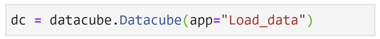
The datacube.Datacube class provides access to the datacube. We usually call objects of this class dc, as we have done here. The app parameter is a unique name for the analysis which is based on the notebook file name.

When the cell has finished running, it will show a [2] next to it, and generate a new blank cell below it.

Load Landsat 8 data

This exercise will load Landsat data for an area of Dar es Salaam, Tanzania. We will use a pair of latitude coordinates (-6.90, -6.70) and a pair of longitude coordinates (39.20, 39.37) to specify the area to load. Data will be loaded for the rectangle defined by these coordinate ranges.

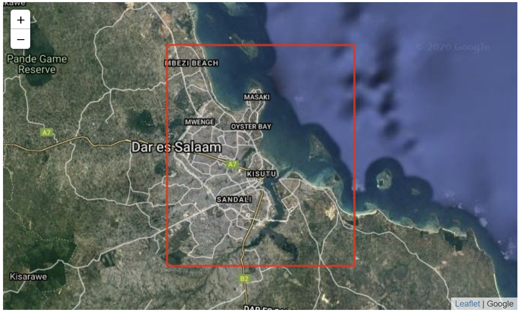
First, we will view this area on a map. This allows us to check we have the correct coordinates. In the new cell below, enter the following code, and then run it to see this area on a map.

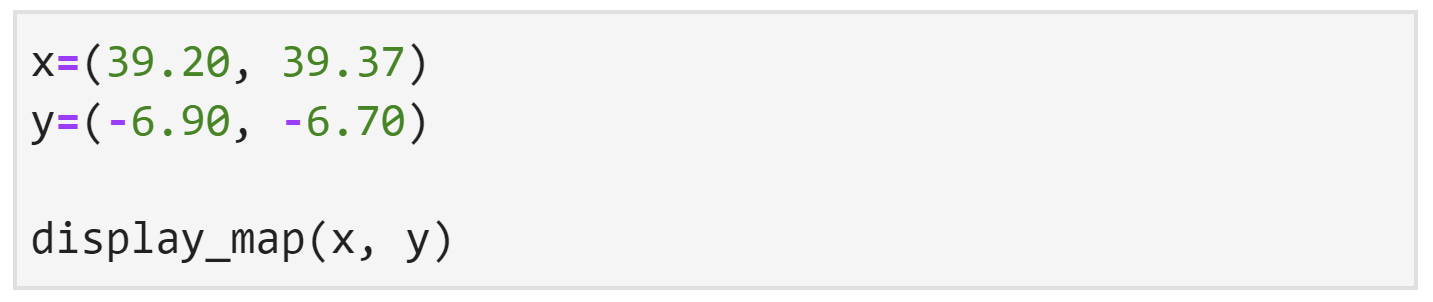
The output of that cell should look like this.

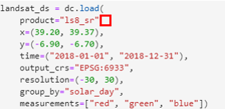
In the new cell below, enter the following code, and then run it to load Landsat 8 data.

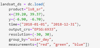
We load data with the dc.load() function. We have chosen to call the loaded dataset landsat_ds. The text between the brackets of dc.load() are our parameters. We have chosen to put the parameters on separate lines to make the code easier to read (and errors easier to spot). Each parameter must be separated by a comma.

• The product argument is the datacube product to load data from. We want to access the Landsat 8 dataset, which is named ls8_sr.

  ls8_sr uses only numbers and lowercase letters. It stands for Landsat 8 Surface Reflectance.

• The x and y arguments specify the area to load data for. In this case, they represent longitude and latitude. This defines a rectangle spanning their ranges of coordinate values as seen in the display_map output above.

• The time argument specifies the time range of data to load. We have specified all of the year of 2018.

• The output_crs argument specifies the Coordinate Reference System (CRS) to load data in. The CRS EPSG:6933 specifies an equal area projection — each pixel has the same area.

• The resolution argument is the y and x resolutions (in that order) in pixels per degree. The first value is typically negative. In this case, a resolution of (-30, 30) is a resolution of 30 metres per pixel, which is the maximum resolution of Landsat data.

• The group_by argument controls how data that is close in time is combined to provide better images. Specifying a value of 'solar_day' is recommended.

• The measurements argument specifies what bands will be loaded. We will plot a true-colour image of this data later. To do that, we need the red, green, and blue bands.

Note

As of June 2021, DE Africa Landsat data has been upgraded to Collection 2. Datacube names have been updated to ls5_sr, ls7_sr and ls8_sr. Deprecated naming conventions such as ls8_usgs_sr_scene will no longer work. For more information on Landsat Collection 2, visit the DE Africa Landsat documentation.

Troubleshooting code

Sometimes, typing mistakes can occur. This will produce an error message when you run the cell.

For example, this error is a SyntaxError.

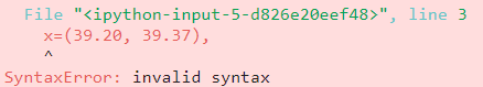
It tells us there might be a mistake just before the section of the code x=(39.20, 39.39),. Sure enough, this error message was generated when a comma was missing after the product parameter, as shown in the screenshot below.

For illustrative purposes, the point where the comma is missing has been highlighted by a red box, but this will not appear in JupyterLab — you will have to find the error or errors yourself.

If errors such as IndentationError or SyntaxError appear, they must be resolved before you can continue. Try checking for some of these common issues:

• Are all brackets and quotation marks in the right place?

• Does every open bracket have a corresponding close bracket?

• Do your bracket types match? ( must be closed by ) and [ with ], and they have different meanings in Python, so they are not interchangeable.

• Does every opening quotation mark have a closing quotation mark? You can use either ' or ", but pairs of quotation marks must be the same.

• Are there commas , between items listed in square brackets [] or parentheses ()?

• Is the indentation correct? Press Tab on your keyboard to increase the level of indentation, and press Shift + Tab on your keyboard to decrease the level of indentation.

• Is everything spelt correctly?

Once you have made your changes, try executing the cell again, by pressing Shift + Enter on your keyboard.

If you get a NameError, it could be because you have not yet imported the required packages and functions. They must be imported every time you start a new server session. To resolve this, follow the instructions in the section above, Load packages and functions.

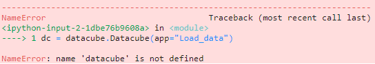
An example of a NameError caused by not importing the datacube package.

Note

Take your time to type code. If you would like to learn more about Python code syntax, or more chances to practise basic Python skills, take a look at the optional extra session Python basics.

Examine data

When the dc.load() cell successfully executes, it will create a new cell below it. In this new cell, we can enter the name of our dataset and run the cell. This will show the dataset we loaded.

The output of the cell should look similar to this:

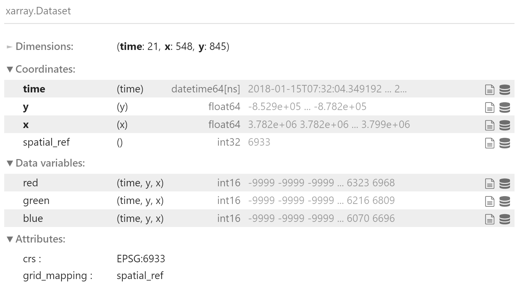
The output of dc.load() is an xarray.Dataset object. This type of dataset is a common format for satellite data, and is organised by:

• Dimensions: The dimensions of the dataset. For Earth observation data, this is often x (longitude), y (latitude) and time, as seen here. The units for the x and y dimensions are pixels, while time is counted in number of flyovers. In this example we see there were 21 flyovers of our selected location during the year of 2018.

• Coordinates: A list of the values of each dimension. spatial_ref refers to the CRS we selected in dc.load().

• Data variables: The data values for our chosen measurements. We see red, green and blue are loaded as we specified in the dc.load() command. This product provides values for surface reflectance, which is unitless.

• Attributes: Metadata about this dataset. The CRS is listed again.

Plot a true-colour image

True-colour images are also known as red-green-blue (RGB) images. They are rendered using the image’s ‘natural’ colours and appear how they might be seen by the human eye. As we loaded red, green and blue bands from Landsat 8, we can now plot an RGB image using the data from landsat_ds.

In the next blank cell, enter the following code. Run the cell to generate an RGB image.

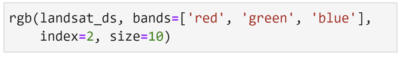
The function used here is called rgb().

• The first item inside the rgb() brackets is the name of the dataset we are drawing the data from. In this case, we want to pull information from landsat_ds.

• bands specifies the name of the data variables in the dataset that correspond to red, green and blue. We saw above that in landsat_ds they are conveniently named red, green and blue.

• index refers to the timestep to view. The default is 0. The Python language counts from 0, so index=0 shows the first flyover, and index=1 the second.

• size is the height of the image.

The RGB image will look like this:

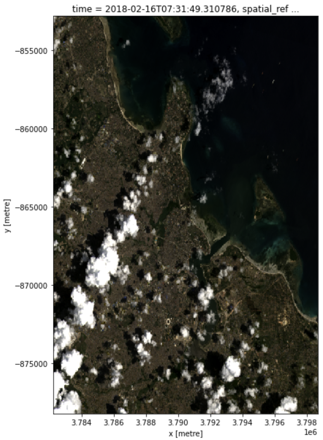
The title of the image notes that the date for this data is 2018-02-16, or 16 February 2018.

Exercise: Load and plot Sentinel-2 data

Let us repeat the data loading process for Sentinel-2 data. It is a very similar process to loading the Landsat 8 data. We want to load data for the same time and place, so we only have to change the product and resolution.

1. Let us call our Sentinel-2 dataset sentinel_2_ds. You must name it something different from the Landsat 8 dataset. In a new cell, type the name of the Sentinel-2 dataset.

   

2. Again, we will use dc.load() to import Sentinel-2 data. After sentinel_2_ds, type = dc.load(). It should look like sentinel_2_ds = dc.load().

   How do we fill out the parameters inside the brackets of dc.load()? We can do this by copying some of the information from the Landsat 8 dc.load() input cell. The first parameter we listed before was product. However, we don’t want to use the Landsat 8 product, we want to select the Sentinel-2 product, s2_l2a.

   

Note

s2_l2a stands for Sentinel-2 Level-2A. The fourth character is a lowercase alphabet ‘l’. Double-check you have entered the product name correctly to avoid errors.

3. The resolution parameter will also be different from the Landsat 8 load. For Sentinel-2, it should be (-10,10), since our Sentinel-2 data has a resolution of 10 metres per pixel.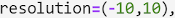

   

4. Now, type the rest of the parameters to be the same as they were for the Landsat 8 load. This includes:

   • x

   • y

   • time

   • output_crs

   • group_by

   • measurements

   As before, watch out for commas, quotation marks, and brackets to avoid error messages when running the cell.

5. You should end up with a set of parameters that look like this:

   

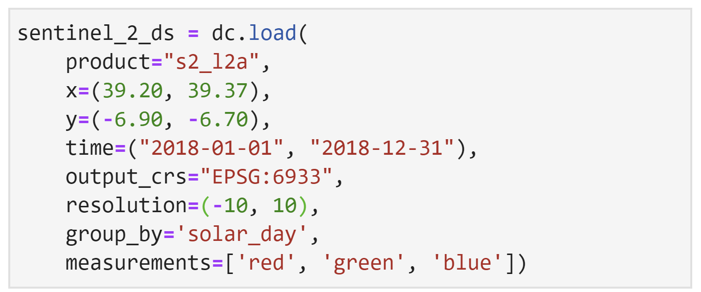
6. Run the cell to load Sentinel-2 data.

7. In the new cell below that, let us plot an RGB image around the same time as the Landsat 8 RGB image, which was from February 16, 2018.

   We must specify the dataset first, followed by the bands, index, and size. In this case, we want to use index=9. Ensure the cell has the following code and then run it.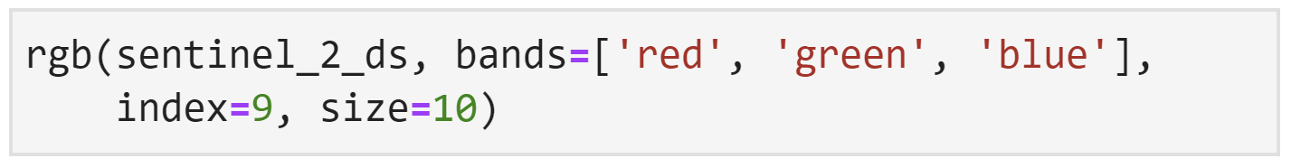

   

8. An RGB image using Sentinel-2 data will be generated.

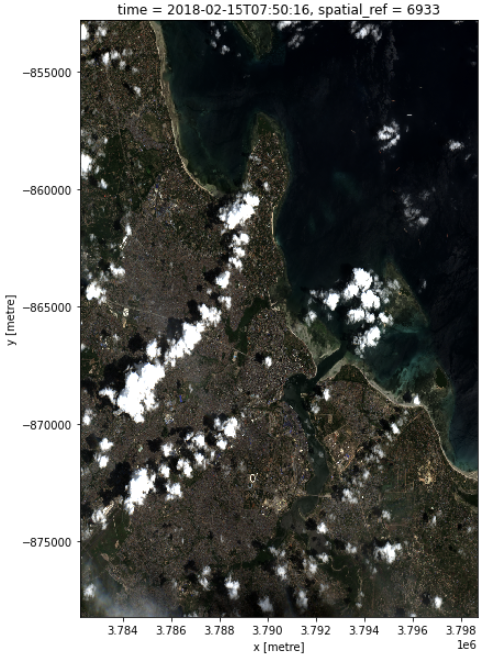
As Landsat 8 data and Sentinel-2 data come from different satellites, their flyovers are not always at the same time. In this case, the closest date of Sentinel-2 data to the Landsat data is one day before, on February 15, 2018. It is another cloudy scene, like the Landsat 8 one.

Conclusion

You have successfully loaded and plotted data for Landsat 8 and Sentinel-2.

You have also finished the second session of the Digital Earth Africa training course. In this session, you have learned about:

• Digital Earth Africa products, including Landsat 8 and Sentinel-2

• Visualising data with the Digital Earth Africa Map

• Exploring data availability with the Digital Earth Africa Explorer

• Loading data in the Sandbox

• Generating RGB images

Congratulations!