Running a Notebook

Now that you have learned to open and close notebooks, this section will teach you how to run an analysis using one of the existing Jupyter notebooks.

Overview

Jupyter is an interactive coding environment compatible with the programming language Python. Digital Earth Africa is based on a Python library called the Open Data Cube, so the Sandbox contains Python-based notebooks.

It is helpful, but not required, to be familiar with Python programming. More detail on Python can be found in Extra session: Python basics, which is an optional module that provides greater context into common Python commands used in the Digital Earth Africa platform. It is recommended to first follow the steps below to set up a folder in the Sandbox environment before completing the Python basics module.

Video: Working with notebooks

This video gives an overview of the notebook we will be working with. Watch the video, and then follow the written instructions below to complete the exercise.

Exercise: Run the Crop Health notebook

This activity will demonstrate how to run one of the Digital Earth Africa Sandbox notebooks. The notebook is a real world example showing how to measure crop health. Follow the instructions below to run the notebook.

Create a copy of the notebook

The Sandbox comes with a large number of existing notebooks, which you can use as reference material. To keep these in their original format, we recommend making a copy of a notebook when you want to run it. For the rest of this training material, we will ask you to make copies of notebooks and store them in a new Training folder. Follow the instructions below to set up this folder and add a copy of the notebook for this session.

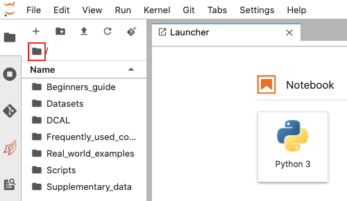
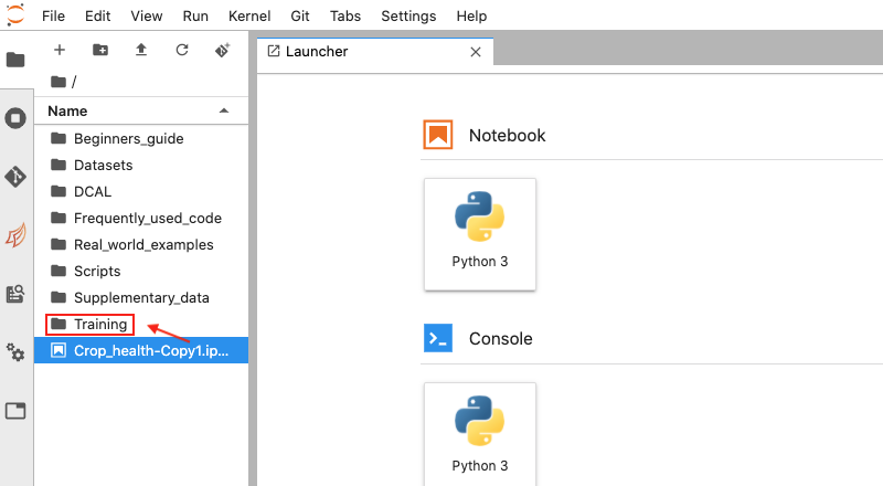
1. Click the Folder icon in the folder path to make sure you’re in the Home folder.

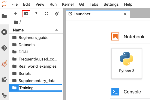
2. Click the New Folder icon and name the new folder Training. Press Enter to finish creating the folder.

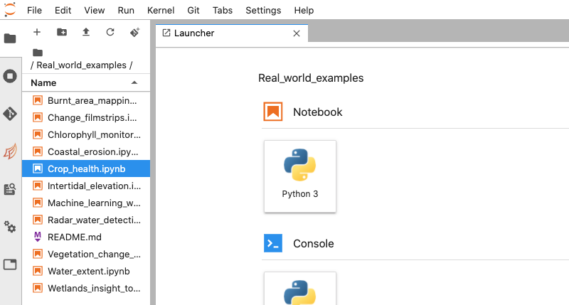
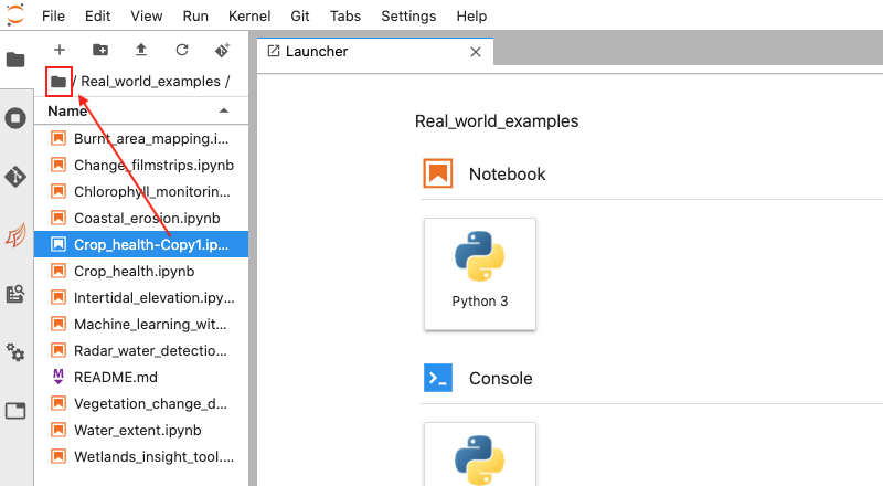
The next step is to identify and copy the notebook you want to work on. For this exercise, this will be the Crop_health.ipynb notebook, which is in the Real_world_examples folder. Follow the steps below to copy it.

3. Double-click the Real_world_examples folder to open it. The Crop_health.ipynb notebook is selected in the image below.

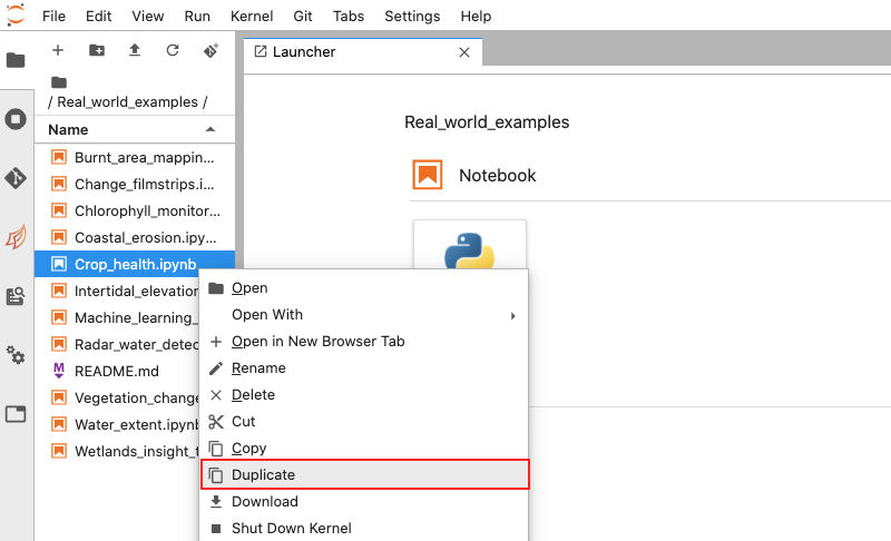
4. Next, right-click on the notebook and click Duplicate to create a copy. By default, this will be called Crop_health-Copy1.ipynb.

5. Click and drag Crop_health-Copy1.ipynb to the Folder icon to move it to the Home folder.

6. Return to the Home folder by clicking the Folder icon. You should see the Crop_health-Copy1.ipynb notebook. Click and drag this file to the Training folder you created.

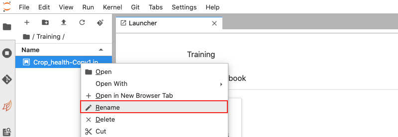
7. Double-click the Training folder. Right-click the copied notebook and click Rename. Rename the notebook to Crop_health.ipynb.

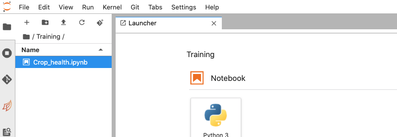
You can now run this notebook, as well as make edits to it.

Starting the notebook

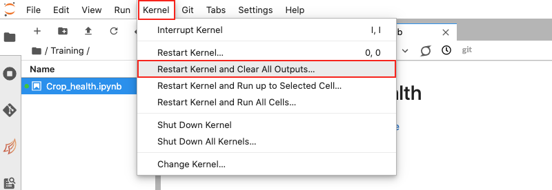
Notebooks on the Sandbox come pre-run. It is best practice to restart and clear the notebook before running.

1. Double-click your copied Crop_health.ipynb notebook to open it.

2. In the main menu, click Kernel -> Restart Kernel and Clear All Outputs. When asked whether you want to restart the kernel, click Restart.

3. Read the Background and Description sections to learn more about the notebook.

Loading packages and functions

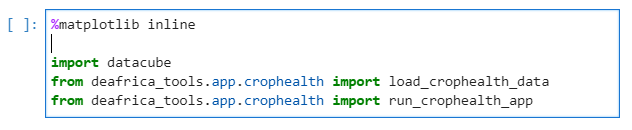
This notebook uses Python packages and functions to conduct the analysis. These are contained in the first code cell, which looks like:

To load the necessary packages and functions:

1. In the Crop_health.ipynb notebook, click on the code cell that matches the one above.

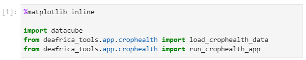
2. Press Shift + Enter on your keyboard to run the cell.

3. When the cell has finished running, the [ ] icon to the left of the cell should change to [1], as shown below. This indicates that the cell has finished running. The number 1 indicates that this was the first cell run in the notebook.

Pick a study site

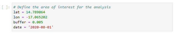
Next, we have to provide the area of interest using latitude, longitude, and a buffer, which describes how many square degrees to load around the set latitude and longitude values. We also set a date. Data from two years up to this date will be loaded.

For now, keep the values that have been set. The notebook will turn this into a bounding box, which will be used to load the data.

1. Click on the cell corresponding to the image below in the notebook.

2. Press Shift + Enter on your keyboard to run the cell.

3. When the cell has finished running, the [ ] icon to the left of the cell should change to [2].

Loading the data

This notebook uses a special function called load_crophealth_data to load the required data. Later in this training course, you will learn how to write your own data loading commands.

The cell containing this function is shown in the image below:

The load_crophealth_data function goes through a number of steps. It identifies the available Sentinel-2 data over the last two years, then masks the bad quality pixels such as cloud and cloud shadow. After the masking step, the function only keeps images where more than half the pixels are good. Finally, it calculates the Normalised Difference Vegetation Index (NDVI) and returns the data. The returned data are stored in the dataset object.

To run the cell:

1. Click on the cell corresponding to the image above in the notebook.

2. Press Shift + Enter on your keyboard to run the cell. Outputs should start to appear below the cell.

3. When the cell has finished running, the [ ] icon to the left of the cell should change to [3].

As the cell is running, you should see outputs describing the function’s actions. The output is shown in the image below:

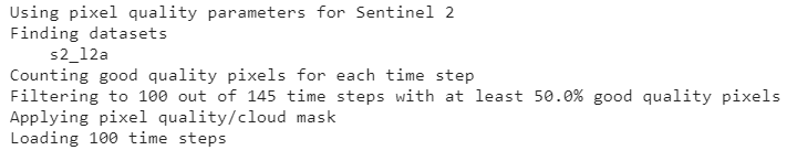
In this case, the function identified 145 observations over the last 2 years, then kept and loaded 100 that met the quality requirements.

Run the Crop Health App

After loading the data, you can visualize the health of various fields using the run_crophealth_app function. This is a special function for this notebook, which takes the dataset you loaded, as well as the latitude, longitude and buffer parameters that define the area of interest. It then starts an interactive app that you can use to measure the average NDVI in different fields.

The cell containing this function is shown in the image below:

1. Click on the cell corresponding to the image above in the notebook.

2. Press Shift + Enter on your keyboard to run the cell. An interactive app should appear, as shown in the image below:

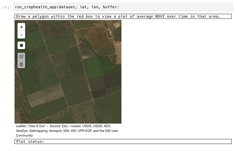
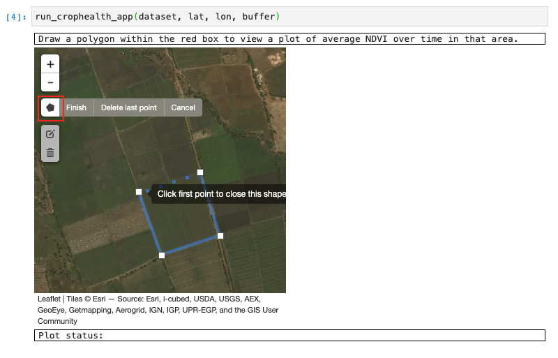
3. The left-hand side of the app contains a map, which will allow you to draw a polygon around a field of interest. Click the Polygon icon, then click points on the map to outline an area, as shown below:

Note

The map in this app shows an ESRI basemap which is higher resolution than the Sentinel-2 data used to calculate the NDVI index. The purpose of the map is to guide you in drawing field boundaries.

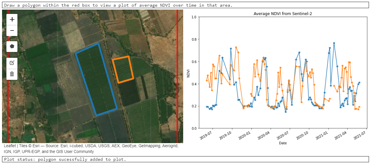
4. Click the first point of the polygon to finish selecting the area. The app will then calculate the average NDVI for that area and display it on the right-hand side of the app, as shown below:

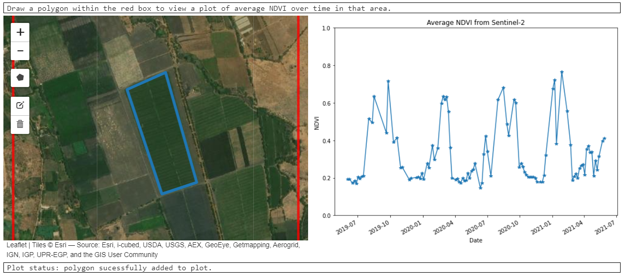
The cycles in the graph are likely related to growth and harvesting events.

5. It is possible to draw multiple polygons and compare the vegetation index over time of different fields. Click the Polygon icon to draw a second polygon:

Conclusion

Congratulations! You have finished the first session of this training! You now know how to open and close notebooks, make copies of notebooks and run them.

Optional activity

If you would like to re-run this notebook using a different area of interest, follow these steps:

1. Restart the notebook and clear all outputs.

2. Run the cell that imports packages and fuctions.

3. Change the latitude, longitude and buffer values in the second code cell. You can either use the values suggested above the cell, or provide your own. Then run the cell.

Note

If you’re going to use your own area of interest, make sure data is available by looking at the Sandbox Metadata Explorer for Sentinel-2 at https://explorer.digitalearth.africa/s2_l2a. You will also need to make sure you provide latitude and longitude values (rather than Easting and Northing values).

4. Run the rest of the notebook as described in the tutorial, drawing in areas of interest using the Polygon icon on the map. Did you learn anything interesting about the fields for your area of interest?

5. Investigate the optional Python basics extra session before continuing on to Session 2. If you are new to Python, it may be helpful for context and reference. If you have previous experience in Python, it provides a review of the major concepts used in the Digital Earth Africa training course.