Create a geomedian composite
This exercise follows on from the previous section. In the previous section, we loaded Sentinel-2 data using load_ard(). This applied a cloud mask to the data by identifying and removing cloudy data points. We can now use this data to create a geomedian composite.
In this section, we will re-run the notebook from the previous section, and extend it to create a geomedian composite. First, we will open and run our Geomedian_composite.ipynb notebook. This will ensure it loads the Sentinel-2 cloud-masked data. Then, we will use a function called xr_geomedian to calculate geomedians. This will allow us to plot a cloud-free geomedian composite image.
Note
We will be using the notebook we created in the previous section, Cloud masking with load_ard(). If you have not already set up a notebook called Geomedian_composite.ipynb with the required packages and functions, follow the instructions in previous section. Ensure you have completed all the steps, including loading the Sentinel-2 dataset for the Ghanaian coast.
Open and run notebook
If you are following directly on from the last section, you can skip this step. If you have closed your Sandbox browser tab or disconnected from the Internet between exercises, follow these steps to ensure correct package imports and connection to the datacube.
Navigate to the Training folder.
Double-click
Geomedian_composite.ipynb. It will open in the Launcher.Select Kernel -> Restart Kernel and Run All Cells…
When prompted, select Restart.
The notebook may take a little while to run. Check all the cells have run successfully with no error messages.
Check the Sentinel-2 dataset
Let’s confirm we have successfully loaded our Sentinel-2 dataset. Recall we named it sentinel_2_ds. Scroll to the bottom of the notebook and run the dataset name in the next empty cell.
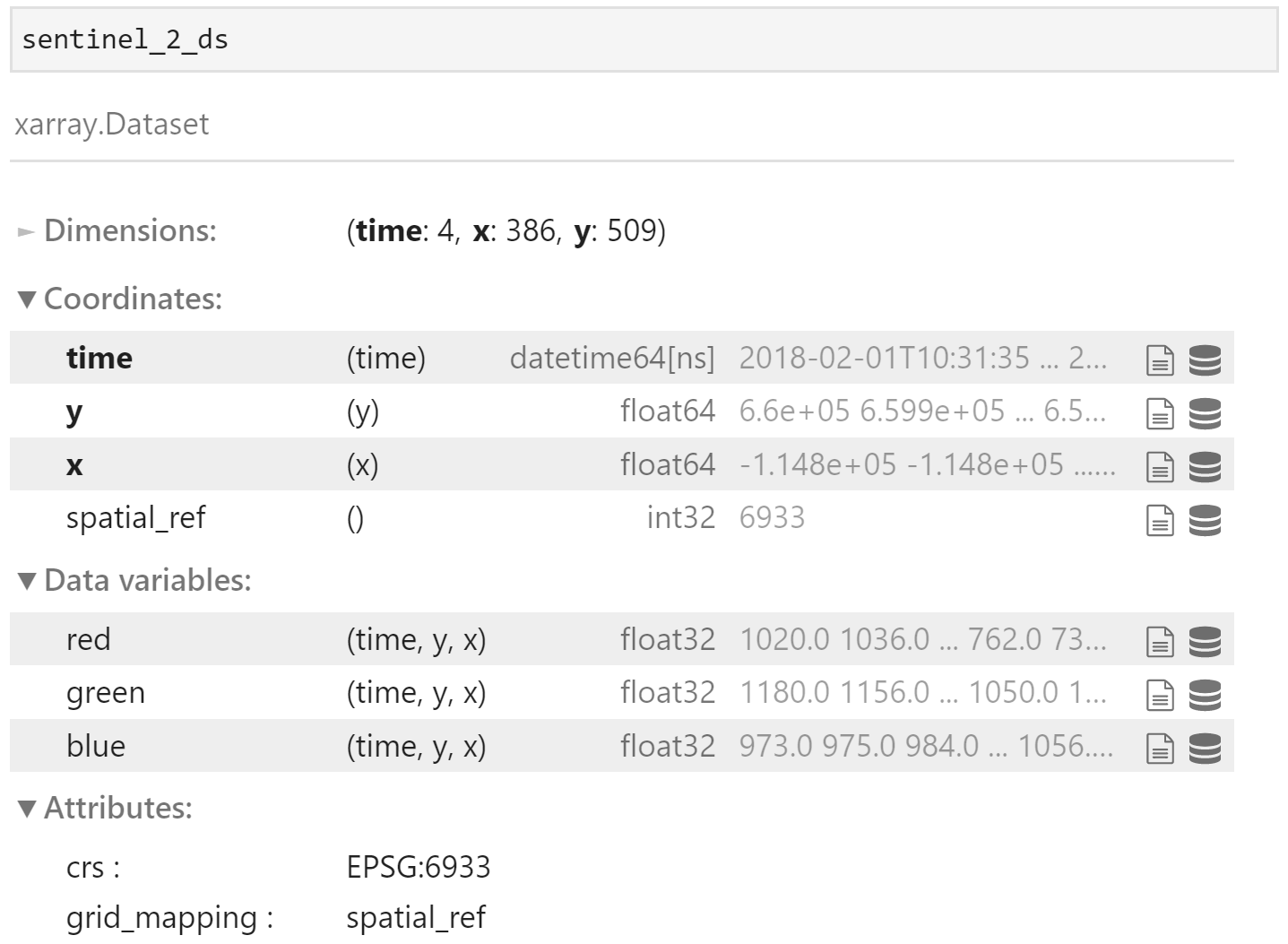
The output should show we have 4 timesteps.
Note
If you encounter a NameError error message, you might need to reload your packages and functions. Follow the steps above, under Open and run notebook.
Create a geomedian composite
Now we will create a geomedian composite using the xr_geomedian function. In the next empty cell below, enter the following code, and then run it.

This generates a dataset called geomedian_composite which contains one geomedian value for every pixel.
Create an RGB image of the composite
In the new cell below, enter the following code, and then run it to generate an RGB image of the composite.
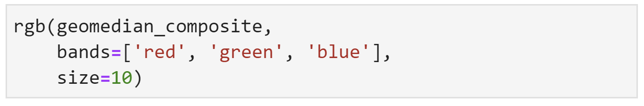
The RGB image will look like this:
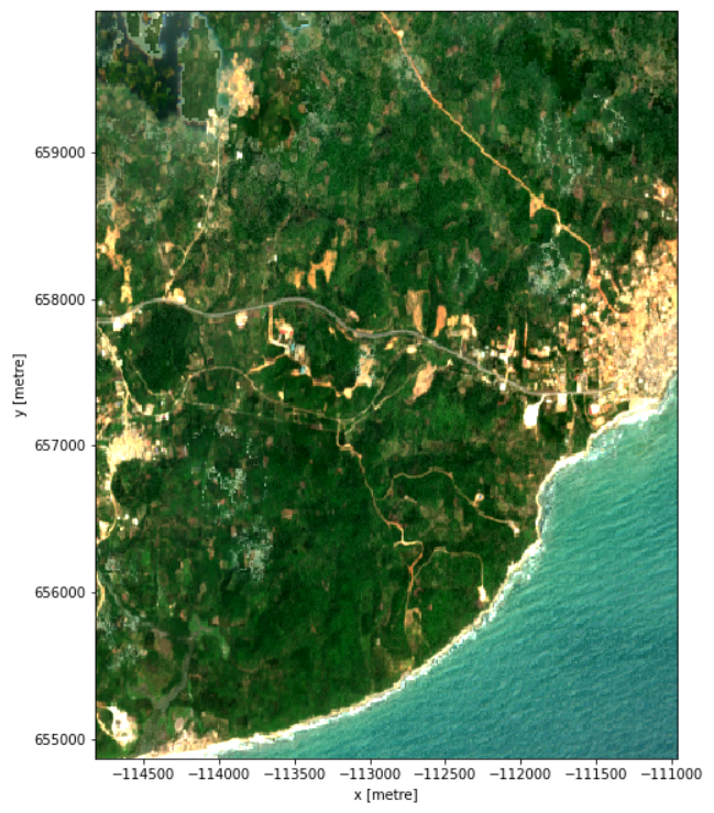
Excellent! There are no clouds or cloud shadows in the geomedian composite.
There are some visual anomalies, but most of the image accurately represents the area. Note that this image is a representation of what the area looked like over the loaded time range, so from 1 February, 2018, to 15 March, 2018.
Note
Save your work by clicking File -> Save Notebook or pressing Ctrl + S.
Conclusion
We have created a geomedian composite of Sentinel-2 data and seen that it is an accurate representation of an area. It fills in missing or masked data, such as clouds and cloud shadows.
This is the end of Session 3. In this session, you have been introduced to the concept of using composite datasets and images to fill in data gaps. We have also learned the best statistical method of combining datasets is the geomedian. Good work!