Introduction to cloud-free composites

Overview

This session is about creating representative datasets and images from multiple timesteps. This allows us to remove and replace unwanted data, such as clouds, and also form images that accurately represent the area of interest over a period of time.

This is summarised in this week’s video, Time aggregation of data. Watch the video to see how to use Earth observation data at different points in time.

Video: Time aggregation of data

Download the video slides as a PDF

In the video, we saw that we can compensate for missing or cloudy data points by using data from different points in time to fill in the gaps. This is a two-step process:

1. Identify and remove cloudy data — this is known as ‘cloud masking’

2. Use data from a different time to fill in missing data — this can be done by calculating geomedians

In this section, we focus on why cloud masking is an important step in preparing your dataset, and introduce the easiest way to do this in the Sandbox. We then briefly explain the significance of geomedians compared to other statistical values.

The two pages following this introduction will involve walkthrough exercises, so you can try performing these steps yourself after reading about them in this section.

Recap: loading and plotting data

In the last session, we plotted RGB images for Dar es Salaam in Tanzania. The image had clouds in both the Landsat 8 and Sentinel-2 versions.

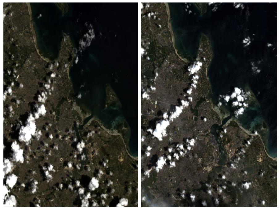
Landsat 8 data from 16 February 2018 (left), and Sentinel-2 data from 15 February 2018 (right). Some cloud cover is visible in both images.

What if we want to know what is underneath those clouds? If you have data at only one point in time, this is not possible. However, if we have data for the same place at a different time, when the clouds are not present, we can use this data to ‘fill’ in areas of cloud.

To do that, we must first identify which pixels are clouds. The process of determining and removing cloud data points is known as ‘cloud masking’.

load_ard() vs dc.load()

The easiest way to apply a cloud mask to your dataset is to load it into the Sandbox using the load_ard() function. ard stands for ‘Analysis-Ready Data’ and the load_ard() function automatically applies a cloud mask.

We previously loaded data in the Sandbox using dc.load(). dc.load() is a universal function for loading data from the datacube and it is important to know how to use it. However, it does not have a built-in cloud masking capability.

When we plotted the RGB images of Tanzania with data loaded using dc.load(), the clouds were part of the image. This makes it difficult to perform cloud masking, as the dataset does not distinguish cloud and not-cloud.

In this exercise, we will instead use the command load_ard() to load our data. It demands similar parameters to dc.load(), but automatically identifies pixels of cloud, and applies cloud masking to the loaded data.

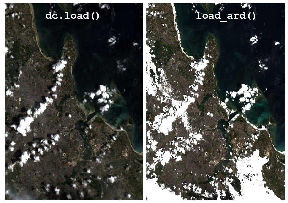
Sentinel-2 data from 15 February 2018 loaded with dc.load() (left) and load_ard() (right). The dc.load image shows cloud cover, while the white pixels in the load_ard image are not clouds, but points where data has been removed by the cloud mask.

The cloud masking algorithm on Sentinel-2 data is more aggressive than its Landsat 8 counterpart. This means it sometimes misinteprets white sand beaches or urban regions as cloud. This can reduce the amount of data available.

Note

load_ard() is compatible with both the Sentinel-2 dataset and the Landsat 8 dataset we used in the last session. However, it is not compatible with some other Digital Earth Africa products, such as Water Observations from Space or GeoMAD, with which you will need to use dc.load().

Calculating a composite

Now that we know how to mask out clouds by using load_ard(), we can load multiple timesteps of our cloud-masked data. These need to be combined in a meaningful way to produce a single image. We do this by compositing our data.

Compositing creates one value for each band for each pixel based on the time series data for that pixel.

We will briefly compare median and geomedian composites, and explain why it is more reliable to use geomedians.

Median composites

For each band in the image, median composites set the value of each pixel to the median value for that band. For a given pixel, each band’s median is independent of the others.

The benefit of a median composite is that it is very fast to compute, so it can be used to quickly create cloud-free images for an area.

However, medians do not account for the fact that every pixel holds information for multiple bands. It is therefore better to use a statistic that is configured for multi-dimensional data, such as a geomedian.

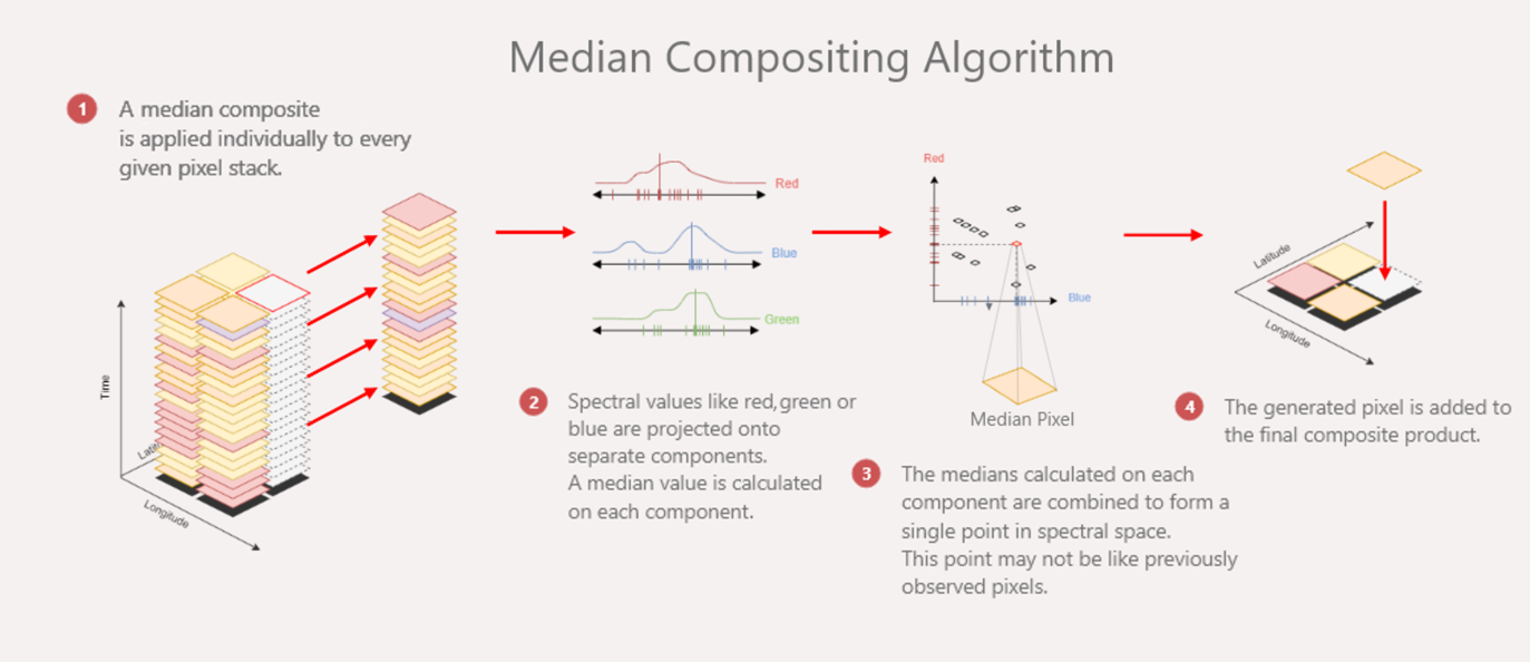
A median considers data from each band independently. This can be seen in Step 2 of the median compositing algorithm shown above.

Geomedian composites

Geomedian — or ‘geometric median’ — composites are multi-band generalisations of median composites. Instead of finding a pixel’s median value for each band individually, like a median composite does, a geomedian composite finds the median values of the bands for each pixel when considered together.

This means they represent the data better than median composites.

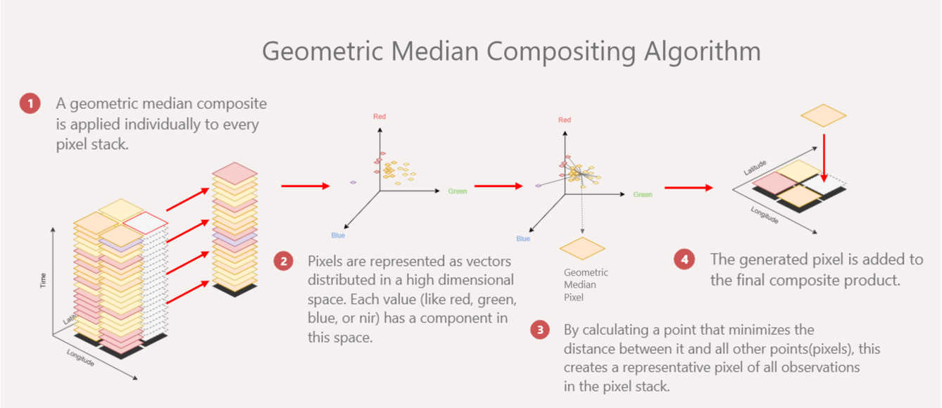
Unlike the median composite, the geometric median (geomedian) considers all bands of data together. Each band adds a dimension to the geomedian calculation. For a three-band dataset, such as the RGB dataset shown in the geomedian compositing algorithm above, each point can be represented on a three-dimensional scatter plot. The geomedian is the minimised ‘sum of distances’ between all the points.

Comparing medians and geomedians

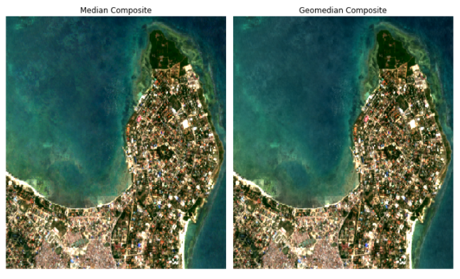
The difference between medians and geomedians can often be subtle, especially if you are looking at the overall composite image. For example, the RGB images for these median and geomedian composites look almost identical.

However, on a pixel-by-pixel basis, it is possible to visualise the difference between median and geomedian. The best way to do this is to use the geomedian widget to explore the effects of different datasets on the median and geomedian.

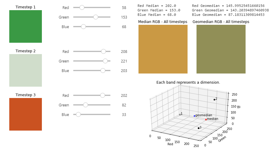
The geomedian widget uses interactive sliders to change the value of the data. This affects the output median and geomedian values. You will soon see that each compositing method can produce significantly different results. On a larger scale (like a whole image, or over several years), this can affect the end composite image.

Download the widget notebook here or visit the Geomedian widget page for for more information, including instructions on running the widget in the Sandbox.

The bottom line: use geomedians

Geomedians take more processing time to calculate than median composites. However, unless you are only doing a quick visualisation, you should use the geomedian method when creating composites. This is because the geomedian value is more scientifically rigorous as it accounts for all the bands in the dataset.

Note

DE Africa produces a pre-computed annual geomedian as part of the GeoMAD service. We will not be using it in this training course, but it produces stunning cloud-free geomedian imagery which can be explored via DE Africa Maps or in the Sandbox. Take a look at the GeoMAD documentation to learn more.

Conclusion

You now know we can perform cloud masking using the load_ard() function, and that we should combine different timesteps of data using a geomedian calculation.

The exercise for this session is covered in the next two sections.

1. We will walk through the process of using load_ard() to load data with a cloud mask.

2. We will then use the loaded data to make and plot geomedians.

This technique will be useful in future sessions for conducting analysis on cloud-free images.