Cloud masking with load_ard()

In this exercise, we will apply a cloud mask to Sentinel-2 data off the coast of Ghana. Cloud masks are important as they remove bad data points from our dataset, so we can form a reliable composite image.

Make a new notebook

Like in the last exercise, we will begin by making a new, blank Jupyter notebook. If you want more detailed instructions on making a new notebook, see this section in the exercise on loading data in the Sandbox from the previous session. Otherwise, follow the steps below.

1. Navigate to the Training folder (or create this folder following the instructions in Session 1).

2. Click the + button and click Python 3 under the Notebook section.

3. Rename your file so you know it is from this exercise. We will use this notebook for working with geomedians, so let us call it Geomedian_composite.ipynb.

4. Open the notebook.

Set up notebook

Load packages and functions

In the first cell, type the following code and then run the cell. Recall that cells can be run by pressing Shift + Enter on your keyboard.

We used most of these packages and functions in the previous exercise on loading data in the Sandbox. rgb is for plotting true-colour images. display_map is for visualising the area we have selected.

In this session we introduce two new functions: load_ard and xr_geomedian. We will use load_ard to load data so it is cloud masked, and xr_geomedian is used in the next section to compute the geomedian.

Note

As of June 2021, the deafrica_tools package has replaced the deprecated sys.path.append('../Scripts') file import. For more information on deafrica_tools, visit the DE Africa Tools module documentation.

Connect to the datacube

Enter the following code and run the cell to create our dc object, which provides access to the datacube.

Your notebook is now set up. Next, we will load cloud-masked data using load_ard().

Load data with load_ard()

Note

If you experience errors when running cells, check out the troubleshooting code guide from the previous session.

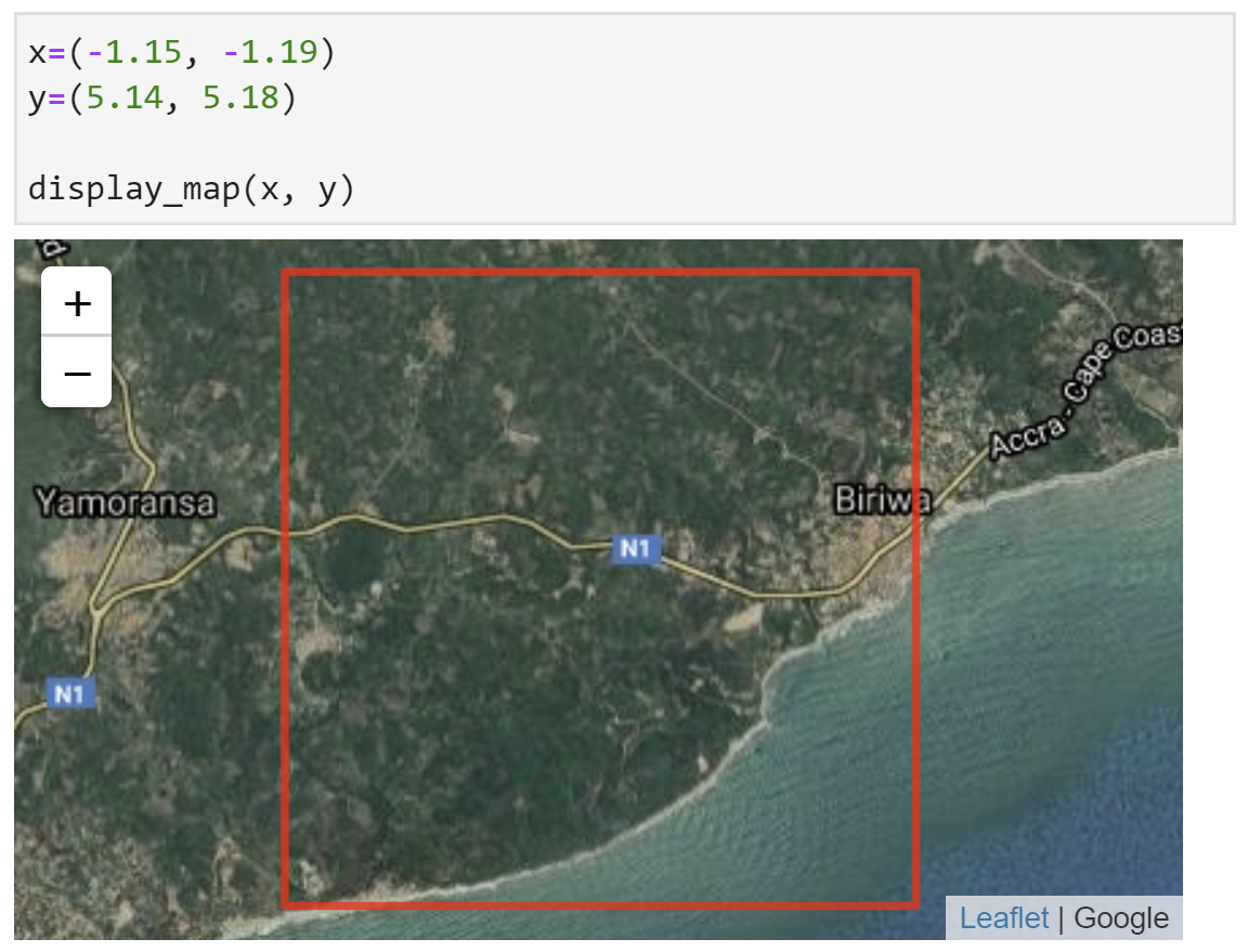
Let us take a look at a coastal area in Ghana. Enter the following code and run it to display a map of the area. As before, x denotes longitude and y denotes latitude.

In the new cell below, enter the following code, and then run it to load Sentinel-2 data. It will generate the output text Using pixel quality parameters for Sentinel 2 .... The output text tells us we have loaded 4 timesteps.

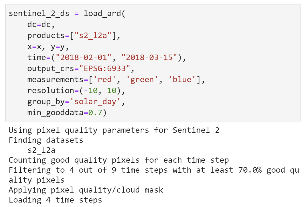
Take note of some of the differences between dc.load() and load_ard.

• dc=dc is a required parameter for load_ard(). This links the data search to the datacube connection, which we defined in the notebook setup as dc.

• The paramter for loading products is products (plural) not product as it is in dc.load().

• Product items must be listed inside square brackets [], which is not required for dc.load().

• min_gooddata stands for ‘minimum good data’ and discards observations with less than the fractional requisite of good quality pixels.

Note

s2_l2a stands for Sentinel-2 Level-2A. The fourth character is a lower-case alphabet ‘l’. Double-check you have entered the product name correctly to avoid errors.

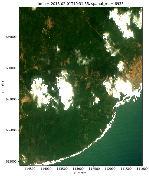
We can use the same rgb plotting code as in the last session to show an RGB image of one of the timesteps. Let’s start with the first timestep, which has an index of 0.

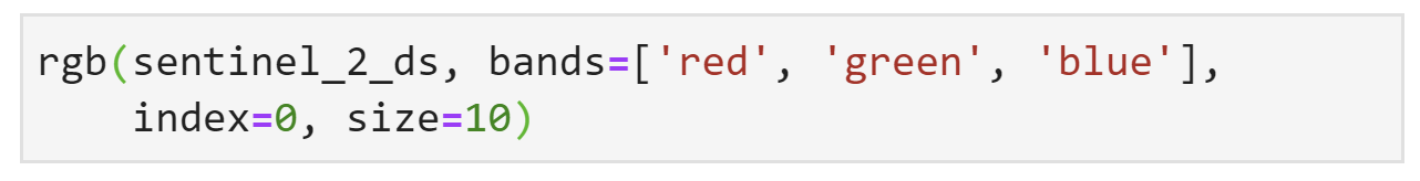
This should produce a single RGB image as shown below. What happens if you try changing the index number?

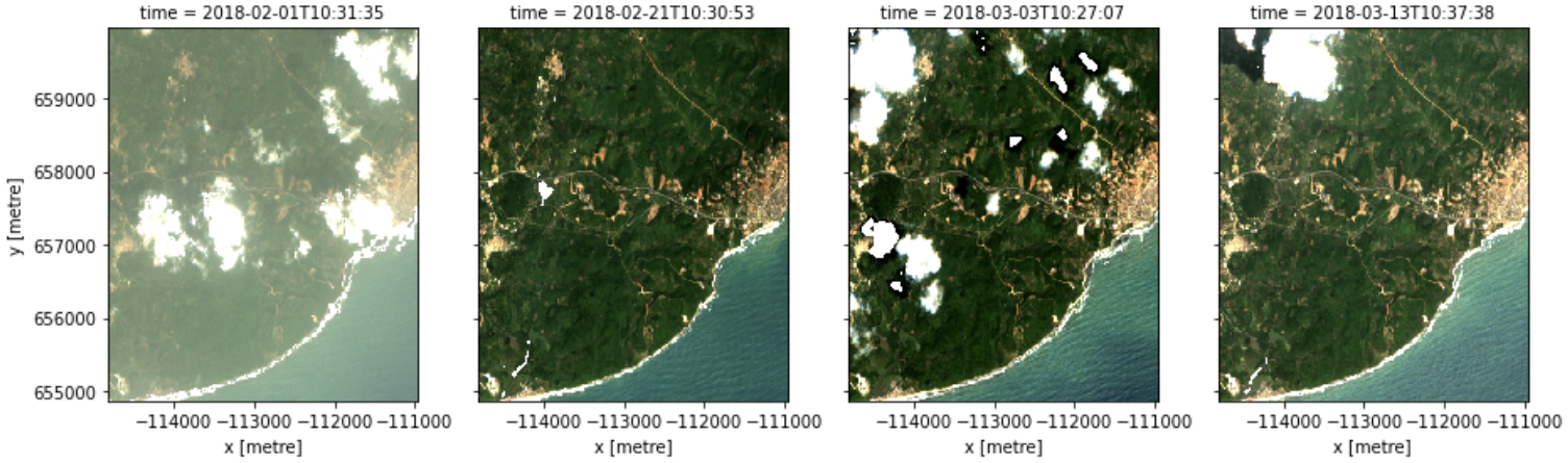
If we want to see RGB images of all the timesteps at once, we can replace the index parameter with the col parameter. The parameter col stands for ‘column’. Specifying col='time' creates a row of images for the timesteps.

The output should look like this.

Conclusion

Good work — you have now loaded data using load_ard(), which has an automatic cloud mask. We can see that the images at different timesteps have different cloud cover, so they have been masked in different places. This is why having data at different timesteps can allow us to create a composite image without any cloud.

In the next section, we will use this loaded data to create a geomedian composite.