Band indices

True-colour images, like the RGB ones we created in Session 2 and Session 3, are an intuitive way of displaying spatial data as it appears to our eyes. However, satellites capture many more layers of data: their range extends outside the visible spectrum. We can also make use of these measurements to perform various kinds of data analysis.

One established analysis technique for identifying specific terrain features, such as water or bare soil, is to calculate a band index.

Video: Band indices

Watch the short video below to learn about band indices. Then, read the text below for more detail.

Download the video slides as a PDF

What is a band?

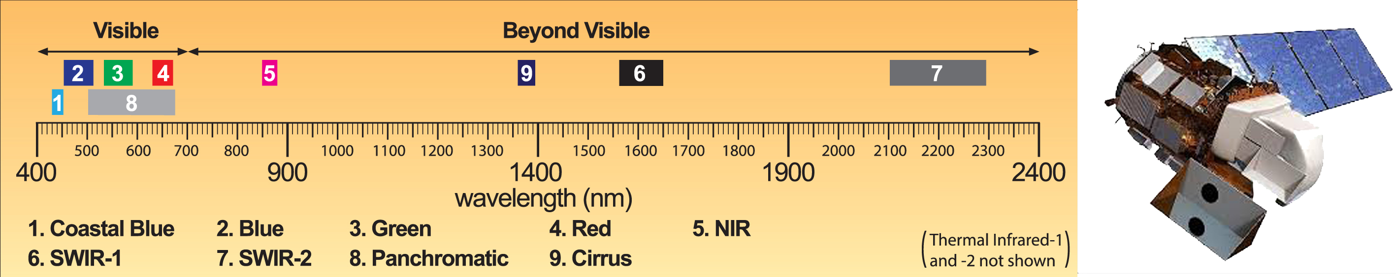
A section of the electromagnetic spectrum showing some of the Landsat 8 bands. [Source]

You may recall from the introduction to satellite products that the range of data acquired by a satellite is defined by its bands. Bands are subdivisions of the electromagnetic spectrum dependent on the sensors on the satellite.

A selection of commonly-used Landsat 8 and Sentinel-2 bands are shown in the table below. We can see the spectral ranges between Landsat 8 and Sentinel-2 are similar, but not the same. Also note the band numbers do not always correspond to the same spectral range.

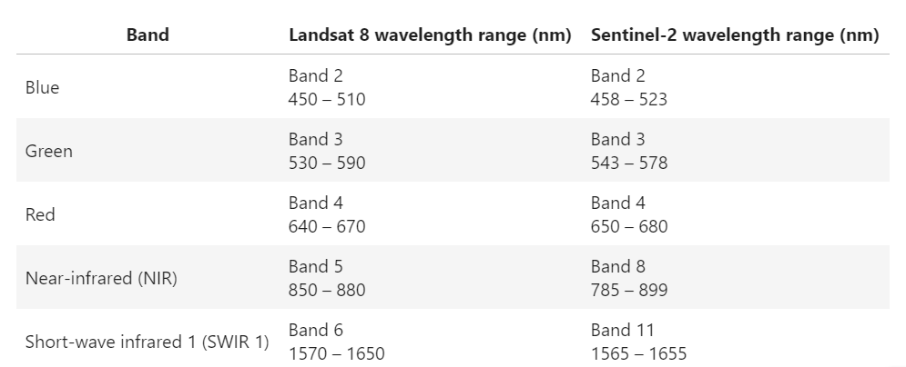
Sources: Landsat 8 bands, Sentinel-2 bands

Bands and terrain features

Different types of ground cover absorb and reflect different amounts of radiation along the electromagnetic spectrum. This is dependent on the physical and chemical properties of the surface.

For example:

• Water: Open water bodies generally reflect light in the visible spectrum, and absorb more short-wave infrared than near-infrared radiation. This can change if the water is turbid.

• Snow: Ice and snow reflect most visible radiation, but do not reflect much short-wave infrared. Reflectance measurements depend on snow granule size and liquid water content.

• Green vegetation: Chlorophyll, a pigment in plants, absorbs a lot of visible light, including red light. When plants are healthy, they strongly reflect near-infrared light.

• Bare soil: The mineral composition of soil can be characterised using the visible and near-infrared spectrum. Soil moisture content can greatly influence the results.

Using these spectral differences, we can calculate ratios between bands to isolate and accentuate the specific terrain feature we are interested in. These metrics are known as band ratios or band indices.

Note

In practice, variation within terrain feature classes, as well as the presence of multiple features in one area, can make different types of ground cover difficult to distinguish. This is one of the challenges of spectral data analysis.

Example: Normalised Difference Vegetation Index (NDVI)

One of the most widely-used band indices is the Normalised Difference Vegetation Index (NDVI). It is used to show the presence of live green vegetation. Generally, green vegetation has a low red band measurement, as red light is absorbed by chlorophyll. In addition to this, healthy leaf cell structures reflect near-infrared light, giving a high near-infrared (NIR) band measurement.

NDVI is therefore typically calculated using a satellite’s NIR band and red band. One value is calculated per pixel.

\begin{equation} \text{NDVI} \ = \ \frac{\text{NIR} - \text{Red}}{\text{NIR} + \text{Red}} \end{equation}

We see the index is calculated by the difference \((\text{NIR} - \text{Red})\) divided by the sum \((\text{NIR} + \text{Red})\). This normalises the index: all values will fall between \(-1\) and \(1\).

Large values of NDVI will occur for pixels where NIR is high and red is low. Conversely, NDVI can be close to 0 or even negative where NIR is low and red is high. This means we interpret NDVI as follows:

\begin{align} \text{NDVI} &> 0, \text{ or close to }1 = \text{green vegetation}\\ \text{NDVI} &\leq 0 = \text{not green vegetation; water, soil, etc.} \end{align}

But what is green vegetation? The US Geological Survey provides a more specific guide to interpreting NDVI.

Areas of barren rock, sand, or snow usually show very low NDVI values (for example, 0.1 or less). Sparse vegetation such as shrubs and grasslands or senescing crops may result in moderate NDVI values (approximately 0.2 to 0.5). High NDVI values (approximately 0.6 to 0.9) correspond to dense vegetation such as that found in temperate and tropical forests or crops at their peak growth stage.

You can see even this definition does not exhaustively cover every kind of vegetation. It is important to remember that Earth observation data analysis is sensitive to the dataset location and time. The nature of climate and environment variations across the globe, and even just within the African continent, mean that band indices like NDVI need to be interpreted with knowledge and context of the area.

Note

Normalising band indices so their values fall between -1 and 1 gives a relative scale that allows for easier data analysis. Values of the index can be better compared between different points in the area of analysis, and across time periods.

Below we have two plots of an area with river distributaries in Guinea-Bissau, a country that experiences monsoonal-like seasons. We see the amount of vegetation as detected by NDVI fluctuates over time. The top image shows NDVI in April, at the end of the dry season. NDVI readings are much lower than when compared to the same area in November (bottom image), after several months of rain during the wet season.

Notice the RGB images may show parts of the area to be visibly ‘dry’ or ‘lush’, but in places where this is less obvious, it is easier to analyse NDVI than the multispectral RGB dataset.

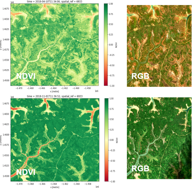
NDVI calculated from Sentinel-2 data in Guinea-Bissau in April 2018 (top left) and November 2018 (bottom left). The NDVI values reflect typical seasonal patterns in a quantitative manner.

Note

We see in the table above that satellites have slightly different band ranges for the same band name (e.g. ‘Red’ for Landsat 8 is slightly different than ‘Red’ for Sentinel-2). This means they will produce different band index values even at approximately the same time and place. It is good practice to compare like datasets only.

Band indices in research

NDVI is just one example of a useful band index. There are many other band indices used in Earth observation research to draw out terrain features. Selecting a band index is often dependent on environmental conditions and research purpose.

• Vegetation: As described above, NDVI is a good baseline vegetation index. It is simple to calculate, and only requires two bands — red and NIR. However, the Enhanced Vegetation Index (EVI) is often more accurate. EVI is calculated with three bands — red, blue and NIR — and requires some coefficients for scaling.

  In arid regions, where vegetative cover is low, consider using the Soil Adjusted Vegetation Index (SAVI), which incorporates a soil brightness correction factor.

• Urbanisation: Human settlements can be identified through urbanisation indices, one of which is the Normalised Difference Built-up Index (NDBI). NDBI uses SWIR 1 and NIR bands:

  \[\text{NDBI} \ = \ \frac{\text{SWIR 1} - \text{NIR}}{\text{SWIR 1} + \text{NIR}}\]

  However, NDBI can be confused between built-up areas and bare soil, so in arid and semi-arid regions where this is problematic, it may be better to use the Dry Bare Soil Index (DBSI).

  \[\text{DBSI} \ = \ \frac{\text{SWIR 1} - \text{Green}}{\text{SWIR 1} + \text{Green}} \ - \ \text{NDVI}\]

• Water bodies: Delineation between water and land can be defined using the Modified Normalised Difference Water Index (MNDWI). It is calculated using green and SWIR 1 bands:

  \[\text{MNDWI} \ = \ \frac{\text{Green} - \text{SWIR 1}}{\text{Green} + \text{SWIR 1}}\]

  This should not be confused with indices for monitoring water content in vegetation.

It is important to remember band indices are not infallible; their usefulness relies on appropriate index selection and sensible interpretation. However, as the field of remote sensing grows, ongoing research into differentiating terrain types with different band combinations give rise to more nuanced and accurate data analysis. For instance, it is common to use more than one index to help distinguish feature classes with similar spectral characteristics.

Conclusion

Band indices are an integral part of spatial data analysis, and are an efficient method of distinguishing different types of land cover. In the following sections, we will calculate NDVI for a cloud-free composite using the Sandbox.