Calculating NDVI: Part 1

This exercise follows on from the previous section. In the final exercise of the previous session, you constructed a notebook to create geomedian composite.

In this section, we will create a new notebook based on the notebook from the previous section. Most of the code will remain unchanged, but we will change the area of interest and time extent. We will also add steps to resample the new dataset and create a geomedian. In the next section, we will calculate and plot NDVI.

Note

We will be using the notebook we created in the previous section, Create a geomedian composite. If you have not already set up a copy of the notebook called Geomedian_composite.ipynb with the required packages and functions, follow the instructions in previous section. Ensure you have completed all the steps, including loading the Sentinel-2 dataset.

Set up notebook

Create a copy of the notebook

Before you continue with the next step,

1. Log in to the Sandbox and open the Training folder.

2. Make a copy of the Geomedian_composite.ipynb notebook.

3. Rename the notebook to Calculate_ndvi.ipynb.

See create a copy of a notebook and rename it for more details.

Clearing the notebook

We will need to remove any output from previous runs of the notebook.

1. Select Kernel -> Restart Kernel and Clear All Outputs….

2. When prompted, select Restart.

Running the notebook

This notebook is still set up to run the Session 3 exercise, so you will need to follow the instructions below to modify it. Work cell by cell and pay attention to what needs to be changed.

Set-up

1. Run the first cell, which contains the packages and functions for the analysis. No need to change anything here.

2. For the dc = datacube.Datacube command, change the app name to "Calculate_ndvi". It should look like:

   dc = datacube.Datacube(app="Calculate_ndvi")
   

Load the data

1. Change the x and y values to those shown below and run the cell.

   x=(-6.1495, -6.1380)
   y=(13.9182, 13.9111)
   

2. Change the time in the load_ard function to ("2019-01", "2019-12").

3. Remove the option min_gooddata=0.7.

   If you completed steps 2, 3 and 4, your load cell should look like

   sentinel_2_ds = load_ard(
       dc=dc,
       products=["s2_l2a"],
       x=x, y=y,
       time=("2019-01", "2019-12"),
       output_crs="EPSG:6933",
       measurements=['red', 'green', 'blue'],
       resolution=(-10, 10),
       group_by='solar_day')
   

4. Run the cell. The load should return 71 time steps.

Plot timesteps

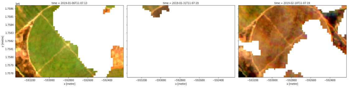
The fifth cell of the notebook contains an rgb command to plot the loaded data. To match our example below, modify this cell so that it matches the code below:

timesteps = [1, 6, 8]

rgb(sentinel_2_ds, bands=['red', 'green', 'blue'], index=timesteps)

This will plot images for the 1st, 6th and 8th timestep of the loaded data (remember that Python starts counting at 0). Your image should match the one below.

Note

You may also like to run this cell a few times, experimenting with different values for the timesteps parameter. The load command should have returned 71 time steps, meaning the values in your timesteps list can be anywhere from 0 to 70.

Resampling the dataset

Resampling is used to create a new set of times at regular intervals. Using the resample method, the data can be arranged in days, months, quarterly (three months) or yearly.

Below gives examples of how the data are grouped.

• 'nD' - number of days (e.g. '7D' for seven days)

• 'nM' - number of months (e.g. '6M' for six months)

• 'nY' - number of years (e.g. '2Y' for two years)

Follow the steps below to resample the dataset time steps to quarterly.

1. Delete the code for plotting all RGB images:

   rgb(sentinel_2_ds, bands=['red', 'green', 'blue'],
   col='time', size=4)
   

2. In the cleared cell, write the following code to resample the data and store it in the resample_sentinel_2_ds variable:

resample_sentinel_2_ds = sentinel_2_ds.resample(time='3MS')

resample_sentinel_2_ds describes how to group the data into quarterly segments. We can now use this to calculate the geomedian for each quarterly segment.

Note

S at the end of '3MS' is to group the data by start of the month.

Compute the geomedian

For this session, instead of calling xr_geomedian(sentinel_2_ds) on the entire array as we did in the previous exercise, we pass the xr_geomedian function to map and apply it separately to each resampled group(resample_sentinel_2_ds).

Replace the existing xr_geomedian code with:

geomedian_resample = resample_sentinel_2_ds.map(xr_geomedian)

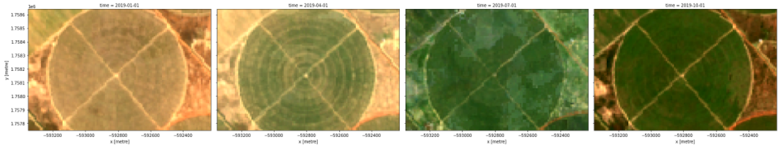
We can plot the output geomedians, and see the change in the landscape over the year. Replace the exsiting rgb code with:

rgb(geomedian_resample, bands=['red', 'green', 'blue'], col="time", col_wrap=4)

Comparing the two datasets

Comparing the two dataset can you tell the difference from the results shown below?

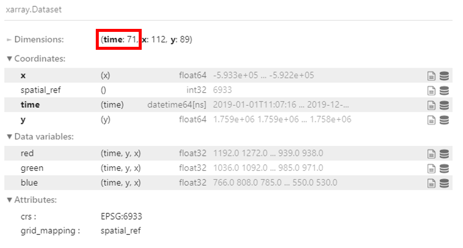
sentinel_2_ds

geomedian_resample

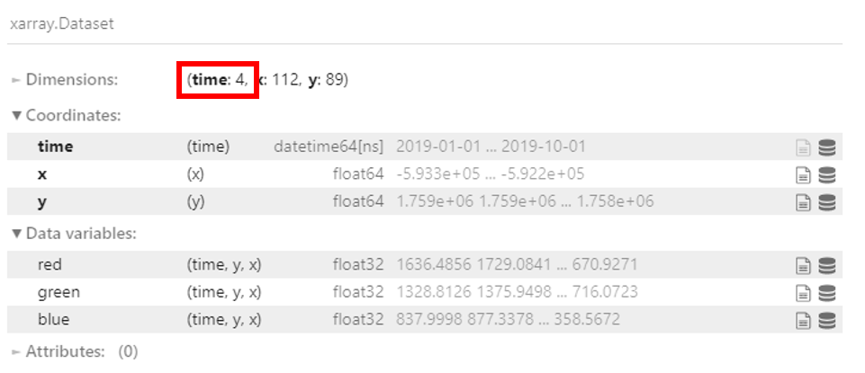
Take a look at the dimensions. The raw dataset sentinel_2_ds has 71 time steps loaded, but after resampling to quarterly as in geomedian_resample, the time dimension is now 4. This makes sense because the year has been divided into four quarters.

Conclusion

Congratulations! You have successfully modified a notebook to create a quarterly geomedian composite by resampling Sentinel-2 data.

If you’d like to experiment futher, try running the code with different resampling values. Did you learn anything interesting to share with us?

In the next section, we will continue working with this notebook to calculate the NDVI values for each of our quarterly geomedians.