Exercise: Vegetation change detection
Overview
In this exercise, we will create a notebook to detect vegetation change. To compare change, we need to have data from two different times: an older dataset, and a newer dataset.
The notebook will include the following steps:
Load Landsat 8 data
Calculate a vegetation index for the loaded data
Split the vegetation index data into half, based on when the data was collected — an older half and a newer half
Compute the mean composite for each half; and
Compare the older and newer averages to check for vegetation change.
At the conclusion of this exercise, you will have performed a vegetation analysis which can be used to report on changes in the selected area.
Set up notebook
In your Training folder, create a new Python 3 notebook. Name it Vegetation_exercise.ipynb. For more instructions on creating a new notebook, see the instructions from Session 2.
Load packages and functions
In the first cell, type the following code and then run the cell to import necessary Python dependencies.
import matplotlib.pyplot as plt
%matplotlib inline

import datacube

from deafrica_tools.datahandling import load_ard
from deafrica_tools.plotting import display_map
from deafrica_tools.bandindices import calculate_indices
Note
As of June 2021, the deafrica_tools package has replaced the deprecated sys.path.append('../Scripts') file import. For more information on deafrica_tools, visit the DE Africa Tools module documentation.
In this exercise, we import one new function, calculate_indices.
Instead of calculating band indices such as NDVI by defining a formula, we can call upon preset index calculations in the Sandbox. calculate_indices contains definitions for over a dozen different indices, from NDVI to the Bare Soil Index (BSI) to Tasselled Cap Wetness (TCW), and can apply them to your dataset.
Using this function to select the index we want might seem like a lot of effort. However, there are some benefits to using the calculate_indices function, as we will see in this exercise.
Reduce chances of error in typing out the formula, as they are already defined in the
calculate_indicesscript — this is great for more complicated formulaeCompare different index results without manually defining many different formulae
Reduce the number of definitions you have to type — for instance, there is no need for
red=ornir=as we used in Session 4
We will use calculate_indices after we load the dataset.
Connect to the datacube
Enter the following code and run the cell to create our dc object, which provides access to the datacube.
dc = datacube.Datacube(app="Vegetation_exercise")
Select area of interest
We need to select an area of interest. Some areas to check for vegetation changes include mining sites, where there might be devegetation, or crops, where seasonal changes in vegetation greenness occur.
Previously, we have provided a longitude range and a latitude range. However, it is more common to define a central point, and provide a buffer around it.
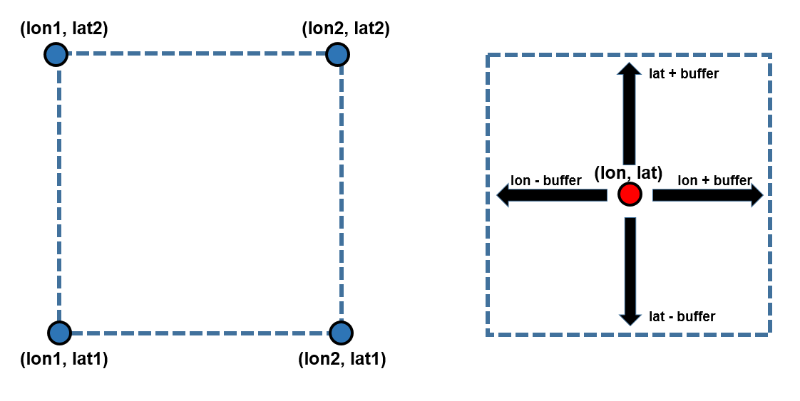
We previously used the x=(lon1, lon2), y=(lat1, lat2) method (left) to define our area of interest. In this exercise, we will use the buffer zone method (right). The advantage is that you can define one buffer to use in all four directions, and it is much easier to explore different areas by changing the central point and/or the buffer width.
We will be selecting an area around a centre point. Enter the following code and run the cell to select an area and time range of interest. The parameters are:
latitude: The latitude at the centre of your area of interest.longitude: The longitude at the centre of your area of interest.buffer: The number of degrees to load around the central latitude and longitude.time: The date range to analyse. For reasonable results, the range should span at least two years to prevent detecting seasonal changes.time_baseline: The date at which to split the total dataset into two non-overlapping samples. For this exercise, we choose a date halfway in our time range. Its value here,'2015-12-31', is halfway between'2013-01-01'and'2018-12-31'- the time range intime. So our two time periods will be 2013 to 2015, and 2016 to 2018.
In the next cell, enter the following code, and then run it to select an area.
# Define the area of interest
latitude = 0.02
longitude = 35.425
buffer = 0.1

# Combine central lat,lon with buffer to get area of interest
lat_range = (latitude-buffer, latitude+buffer)
lon_range = (longitude-buffer, longitude+buffer)

# Set the range of dates for the complete sample
time = ('2013-01-01', '2018-12-01')

# Set the date to separate the data into two samples for comparison
time_baseline = '2015-12-31'
In the next cell, enter the following code, and then run it to show the area on a map. Since we have defined our area using the variables lon_range and lat_range, we can use those instead of typing out (latitude-buffer, latitude+buffer) and (longitude-buffer, longitude+buffer) again.
display_map(x=lon_range, y=lat_range)
Load data
Since we want to look at a longer time range, Landsat 8 data is suitable. In the new cell below, enter the following code, and then run it to load Landsat 8 data.
Notice lat_range, lon_range and time were all defined in the previous cell, so we can use them as variables here.
Note
If you are unsure where we defined lat_range, lon_range and time, scroll up to the previous cell and look for the lines starting with lat_range = ..., lon_range = ... and time = ....
landsat_ds = load_ard(
    dc=dc,
    products=["ls8_sr"],
    lat=lat_range,
    lon=lon_range,
    time=time,
    output_crs="EPSG:6933",
    resolution=(-30, 30),
    align=(15, 15),
    group_by='solar_day',
    measurements=['nir', 'red', 'blue'],
    min_gooddata=0.7)
The output from running the load_ard() function should include a statement that says Loading 46 time steps.
Note
As of June 2021, DE Africa Landsat data has been upgraded to Collection 2. Datacube names have been updated to ls5_sr, ls7_sr and ls8_sr. Deprecated naming conventions such as ls8_usgs_sr_scene will no longer work. For more information on Landsat Collection 2, visit the DE Africa Landsat documentation.
Calculate indices
Now we need to calculate a vegetation index.
Until now, we have used NDVI, which uses the ratio of the red and near-infrared (NIR) bands to identify live green vegetation. The formula is:
This time we will use the Enhanced Vegetation Index (EVI). EVI uses the red, near-infrared (NIR) and blue bands to identify vegetation, and is particularly sensitive to high biomass regions, which is why it can be superior to NDVI. The formula for EVI is more complicated than NDVI as it uses three different bands and some empirical scaling constants.
Instead of typing out that whole formula, we can use the calculate_indices function to calculate EVI. calculate_indices requires three inputs:
The dataset name, e.g.
landsat_dsThe name of the index to calculate, e.g.
index='EVI'The Landsat collection number, e.g.
collection='c2'
c2 stands for ‘Collection 2’, which is the currently-available Landsat collection of data as named by its publishers, US Geological Survey.
In the next cell, enter the following code, and then run it to calculate the EVI vegetation index for this data.
landsat_ds = calculate_indices(landsat_ds, index='EVI', collection='c2')
This adds a variable called EVI to our landsat_ds dataset.
Detect changes
We want to determine what changed in vegetation between the older and newer halves of the data.
First, we will split the vegetation index data into the older half and newer half. Data that was collected in the first half of our time range (2013 to 2015) will go in the older half, and data collected in the second half (2016 to 2018) will be in the newer half.
The split is done using sel() and slice().
sel()stands for ‘selection’ and tells us we are taking a selection of the dataset. We have to define which coordinate we are selecting by. In this case, we will use thetimecoordinate.slice()specifies which part of the coordinate we are taking. In this case, we want to slicetimebetween 2013 – 2015, and then again 2016 – 2018. Recall we named the halfway pointtime_baseline.
We use sel() and slice() to create two new datasets:
baseline_sample: EVI from 2013 to 2015postbaseline_sample: EVI from 2016 to 2018
To do this, enter the following code in the next cell.
baseline_sample = landsat_ds.EVI.sel(time=slice(time[0], time_baseline))
postbaseline_sample = landsat_ds.EVI.sel(time=slice(time_baseline, time[1]))
Here, using time[0] will give us the first date that we stored in the time variable ('2013-01-01'), and time[1] will give us the second date we stored in the time variable ('2018-12-0'). By using the time variable directly, we ensure that the code will work if those dates are changed and the notebook is rerun.
Note
Carefully check all your ., ,, () pairs, and ' ' pairs in the above code to avoid generating errors.
Detect per-pixel changes
Now we have our ‘before’ and ‘after’ datasets, we can compare them for change in EVI. To do this, we will form a composite for each half of the dataset. Then we will calculate the differences in the average EVI for each pixel.
The composite method we are using is the mean (average).
In the next cell, enter the following code, and then run it to create mean composites for the two time periods.
baseline_composite = baseline_sample.mean('time')
postbaseline_composite = postbaseline_sample.mean('time')
Now we need to subtract the first time period EVI mean composite, baseline_composite, from the second time period EVI mean composite, postbaseline_composite. This will determine the change in EVI between the two time periods.
In the next cell, enter the following code, and then run it to determine the change in the vegetation index.
diff_mean_composites = postbaseline_composite - baseline_composite
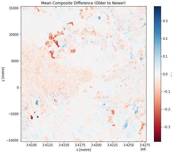
In the next cell, enter the following code, and then run it to show the difference between the mean composites for the time periods. This will allow us to see where the vegetation index increased or decreased and by how much.
plt.figure(figsize=(9, 8))
diff_mean_composites.plot.imshow(cmap='RdBu')
plt.title("Mean Composite Difference (Older to Newer)")
plt.show()
Your plot should look like the image below.
Interpreting the plot
In the code above, the colour for the plot is set using the cmap='RdBu' setting in the diff_mean_composites.plot.imshow() function call. Here, RdBu corresponds to a Red-Blue colour-map, with lower values appearing as red, and higher values appearing as blue.
The areas in blue (positive change) correspond to vegetation increase as measured by EVI. There is more vegetation in these areas in the 2016-2018 sample than the 2013-2015 sample.
The areas in red (negative change) correspond to vegetation decrease as measured by EVI. There is less vegetation in these areas in the 2016-2018 sample than the 2013-2015 sample.
What conclusions can you draw about the changes in the landscape from this plot? What other information might you need to help you assess it?
Conclusion
Congratulations! You have made your own vegetation change detection notebook. It is comparable to the existing Sandbox vegetation change detection notebook. The existing notebook may look daunting, but it includes many of the steps that you have just done! In addition to setting a ‘before’ and ‘after’ scene, the existing notebook:
Plots some true-colour maps (RGB) to inspect the area of interest
Quantifies change using statistical tests (Welch’s t-test for areas of unequal variance)
Identifies statistically significant change
A difference plot, like the one we made above, is a good way to start. You can then decide if you need more complicated analysis or not. You now understand how to structure a complete case study — you can calculate a relevant band index and identify meaningful changes in that index over time.
Optional activity
If you’re curious about how the existing case study works, you can open and run it in the Sandbox:
From the main Sandbox folder, open the Real_world_examples folder
Double-click the Vegetation_change_detection.ipynb notebook to open it
The notebook has already been run, so you can read through it step by step. However, you may find it valuable to clear the outputs and run each cell step by step to see how it works. You can do this by clicking Kernel -> Restart Kernel and Clear All Outputs. When asked whether you want to restart the kernel, click Restart.
There are many similarities between the notebook you built in this session, and the existing Sandbox notebook. Make a note of what is similar and what is different, and spend some time inspecting the different code. If you have any questions about how the existing notebook works, please ask the instructors during a Live Session.