Exercise: Determining the extent of water bodies

Overview

In this exercise, we will create a new notebook to determine the extent of water bodies using the Water Observation from Space (WOfS) product. The WOfS product uses an automated water mapping algorithm to identify water in Landsat 8 images.

The notebook will include the following steps:

• Load the WOfS feature layer product and Landsat 8 data

• Identify water pixels from WOfS

• Plot a true-colour image using Landsat data

• Plot the water body area for the same area using WOfS data

• Customise the plots

At the conclusion of this exercise, you will be able to determine the extent of water bodies using the WOfS product.

Set up notebook

In your Training folder, create a new Python 3 notebook. Name it Water_extent_exercise.ipynb. For more instructions on creating a new notebook, see the instructions from Session 2.

Load packages and functions

In the first cell, type the following code and then run the cell to import necessary Python dependencies.

import numpy as np
import matplotlib.pyplot as plt
%matplotlib inline

import datacube

from deafrica_tools.datahandling import load_ard, wofs_fuser
from deafrica_tools.plotting import display_map, rgb

In this exercise, we import one new function, wofs_fuser. wofs_fuser ensures WOfS data between scenes is combined correctly.

Note

As of June 2021, the deafrica_tools package has replaced the deprecated sys.path.append('../Scripts') file import. For more information on deafrica_tools, visit the DE Africa Tools module documentation.

Connect to the datacube

Enter the following code and run the cell to create our dc object, which provides access to the datacube.

dc = datacube.Datacube(app="water_extent_exercise")

Select area of interest

In the next cell, enter the following code, and then run it to select an area and time. In this exercise, we use a central point and buffer to define our area of interest, similar to what we did in the Session 5 exercise.

The only difference here is that we provide a latitude buffer and a longitude buffer. In this example, they have the same value. However, choosing different buffer values allows you to select rectangular areas of interest, rather than squares.

# Define the area of interest
lat = -6.0873
lon = 35.1817

lat_buffer = 0.2
lon_buffer = 0.2

# Combine central lat, lon with buffer to get area of interest
lat_range = (lat - lat_buffer, lat + lat_buffer)
lon_range = (lon - lon_buffer, lon + lon_buffer)

# Define the year
time = '2018'

Note

Recall code lines beginning with # are comments. They help explain the code, and can be removed or added without impacting the actual Python scripts.

In the next cell, enter the following code, and then run it to show the area on a map. Since we have defined our area using the variables lon_range and lat_range, we can use those instead of typing out (lat - lat_buffer, lat + lat_buffer) and (lon - lon_buffer, lon + lon_buffer) again.

display_map(x=lon_range, y=lat_range)

Create query object

Notice lat_range, lon_range and time were all defined in the previous cell, so we can use them as variables here. We will use them to create a query.

The query variable below is a Python dictionary. It can be used to store parameters. Creating an object variable such as query makes it possible to reuse parameters in various functions that accept the same input parameters.

This is useful to us because we can use it to load the Landsat 8 data, and then use it again to load the WOfS data.

In the next cell, enter the following code, and then run it.

query = {
    'x': lon_range,
    'y': lat_range,
    'resolution': (-30, 30),
    'output_crs':'EPSG:6933',
    'group_by': 'solar_day',
    'time': (time),
}

Note

Notice the structure of the query dictionary is slightly different from dc.load or load_ard. Each parameter name is in quotes '' and is followed by a colon :.

Load data

In the next cell, we load the Landsat and WOfS datasets, naming them ds_landsat and ds_wofs respectively.

In the functions below, we can directly pass the query object using **query — this will give all the settings defined in query to the function.

The main benefit is that we can use the same query for both Landsat 8 and WOfS, which saves us typing it again and prevents us from making mistakes.

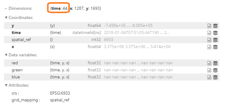
Load Landsat 8

For Landsat 8, we can use the load_ard function.

ds_landsat = load_ard(dc=dc,
                     products=['ls8_sr'],
                     measurements=['red', 'green', 'blue'],
                     **query)

ds_landsat

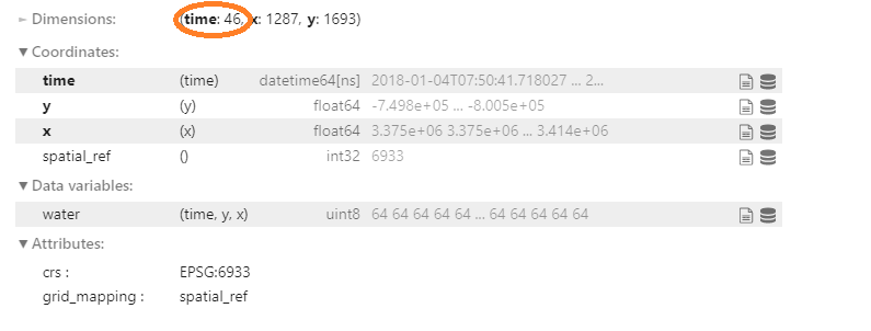
Load WOfS

For WOfS, we need to use the dc.load function.

ds_wofs = dc.load(product=["ga_ls8c_wofs_2"],
         fuse_func=wofs_fuser,
         **query
        )

ds_wofs

Calculating water extent

Understanding the WOfS feature layers

WOfS feature layers are stored as a binary number, where each digit of the number is independantly set or not based on the presence (1) or absence (0) of a particular feature. Below is a breakdown of which decimal value represent which features.

Attribute	Decimal value
No data	1
Non contiguous	2
Sea	4
Terrain or low solar angle	8
High slope	16
Cloud shadow	32
Cloud	64
Water	128

For example, a value of 128 indicates that water were observed for the pixel, whereas a value of 32 would indicate cloud shadow.

In the next cell we will extract only the water features from the WOfS data. This is done by finding values where the water measurement equals 128. In Python, we can find which pixels have a value of 128 by using the == expression:

Extract the water pixels

ds_valid_water = ds_wofs.water == 128

The ds_valid_water array does not contain the decimal values of the WOfS feature layers. Instead, it has a value of False if the pixel was not water, and True if it was water. You can check this by viewing the ds_valid_water DataArray.

ds_valid_water

Calculate the area per pixel

The number of pixels can be used for the area of the waterbody if the pixel area is known. We can extract the size of a pixel from the resolution setting in our query, then divide the area of a single pixel (in square metres) by the number of square meters in a square kilometre.

In Python, number**2 returns the squared value of number.

pixel_length = query["resolution"][1]  # in metres
m_per_km = 1000  # conversion from metres to kilometres
area_per_pixel = pixel_length**2 / m_per_km**2

Calculate area of water pixels

Now that we know how much area is covered by one pixel, we can count up the number of water pixels, and multiply it by this value to get the total area covered by water.

As we saw above, the ds_valid_water array contains True values for water pixels, and False otherwise. When we use the .sum function, it counts True values as 1, and False as 0. Therefore, the sum will be equal to the total number of water pixels for that timestep.

Below, we set the dimensions as x and y to make sure we sum up all the pixels over the spatial dimensions. This means we get one pixel sum for each timestep. This will let us track how the water area changes over time.

ds_valid_water_pixel_sum = ds_valid_water.sum(dim=['x', 'y'])
ds_valid_water_area = ds_valid_water_pixel_sum * area_per_pixel

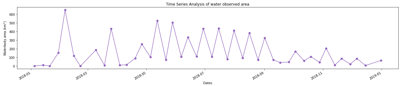
Plot time series

Now that we have the area of water in each observation, we can plot a time series to help us identify dates where the was more or less water within the area of interest.

Below, there is code to set-up, display and customise the plot. The settings are as follows:

• plt.figure(figsize=(18, 4)): set up a figure object to contain the plot, and make it 18 inches long and 4 inches high

• ds_valid_water_area.plot(marker='o', color='#9467bd'): plot the water area data with circular markers in purple (HEX colour code #9467bd)

• plt.title('Time Series Analysis of water observed area'): Give the plot a title

• plt.xlabel('Dates'): Label the x-axis

• plt.ylabel('Waterbody area (km$^2$)'): Label the y-axis. The $ symbols allow the use of LaTeX, a mathematical typesetting language

• plt.tight_layout(): Formats the image so that all axes can be clearly seen

plt.figure(figsize=(18, 4))
ds_valid_water_area.plot(marker='o', color='#9467bd')
plt.title('Time Series Analysis of water observed area')
plt.xlabel('Dates')
plt.ylabel('Waterbody area (km$^2$)')
plt.tight_layout()

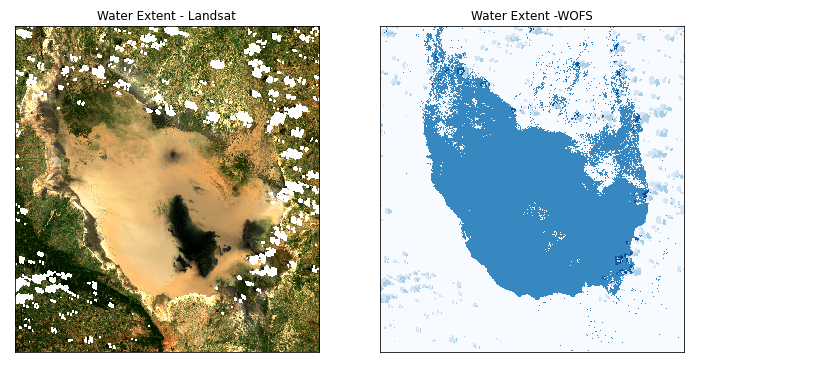
Display of water coverage for a selected timestep

From the graph above you can choose any timestep (between 0 and 45) to display the result on the for both WOfS and Landsat 8.

For example, let us look at the fifth timestep, timestep = 4.

timestep = 4

# Plot water extent
fig, ax = plt.subplots(1, 2, figsize=(12, 6))

#plot the true colour image
ds_nearest_landsat = ds_landsat.sel(time=ds_wofs.time.isel(time=timestep), method='nearest')
rgb(ds_nearest_landsat, ax=ax[0])

# plot the water extent from WOfS
ds_wofs.isel(time=timestep).water.plot.imshow(ax=ax[1], cmap="Blues", add_colorbar=False)

# Titles
ax[0].set_title("Water Extent - Landsat"), ax[0].xaxis.set_visible(False), ax[0].yaxis.set_visible(False)
ax[1].set_title("Water Extent - WOFS"), ax[1].xaxis.set_visible(False), ax[1].yaxis.set_visible(False)

plt.show()

This code uses some additional settings to customise the plot, including allowing to have two plots together. If you want to know more about making this kind of plot, please ask the instructors during a live session.

Try different timestep values — can you find an image where the lake is dried out?

Conclusion

Congratulations! You have made your own water extent notebook. It is comparible to the existing Sandbox water extent notebook.

You’ve now built your second case study! You make like to reflect on what was similar and different between the two. Are there any pieces of code you could reuse for a new analysis? How might you modify your case studies to do more complex analysis?

If you’d like to experiment futher, try running the code with different areas. Did you learn anything interesting to share with us?

Optional activity

If you’re curious about how the existing case study works, you can open and run it in the Sandbox:

1. From the main Sandbox folder, open the Real_world_examples folder

2. Double-click the Water_extent.ipynb notebook to open it

The notebook has already been run, so you can read through it step by step. However, you may find it valuable to clear the outputs and run each cell step by step to see how it works. You can do this by clicking Kernel -> Restart Kernel and Clear All Outputs. When asked whether you want to restart the kernel, click Restart.

Note

If you want to significantly modify it, we recommend you make a copy, like you did in Session 1.

There are many similarities between the notebook you built in this session, and the existing Sandbox notebook. Maybe make a note of what is similar and what is different. If you have any questions about how the existing notebook works, please ask the instructors during a live session.