Python basics 3: Matplotlib

This tutorial introduces matplotlib, a Python library for plotting numpy arrays as images. We will learn how to:

Follow the instructions below to download the tutorial and open it in the Sandbox.

Download the tutorial notebook

Download the Python basics 3 tutorial notebook

Download the exercise image file

To view this notebook on the Sandbox, you will need to first download the notebook and the image to your computer, then upload both of them to the Sandbox. Ensure you have followed the set-up prerequisities listed in Python basics 1: Jupyter, and then follow these instructions:

1. Download the notebook by clicking the first link above. Download the image by clicking the second link above.

2. On the Sandbox, open the Training folder.

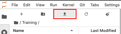
3. Click the Upload Files button as shown below.

4. Select the downloaded notebook using the file browser. Click OK.

5. Repeat to upload the image file to the Training folder. It may take a while for the upload to complete.

6. Both files will appear in the Training folder. Double-click the tutorial notebook to open it and begin the tutorial.

You can now use the tutorial notebook as an interactive version of this webpage.

Note

The tutorial notebook should look like the text and code below. However, the tutorial notebook outputs are blank (i.e. no results showing after code cells). Follow the instructions in the notebook to run the cells in the tutorial notebook. Refer to this page to check your outputs look similar.

Introduction to matplotlib’s pyplot

We are going to use part of matplotlib called pyplot. We can import pyplot by specifying it comes from matplotlib. We will abbreviate pyplot to plt.

%matplotlib inline
# Generates plots in the same page instead of opening a new window

import numpy as np
from matplotlib import pyplot as plt

Images are 2-dimensional arrays containing pixels. Therefore, we can use 2-dimensional arrays to represent image data and visualise with matplotlib.

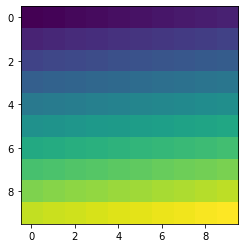
In the example below, we will use the numpy arange function to generate a 1-dimensional array filled with elements from 0 to 99, and then reshape it into a 2-dimensional array using reshape.

arr = np.arange(100).reshape(10,10)

print(arr)

plt.imshow(arr)

[[ 0  1  2  3  4  5  6  7  8  9]
 [10 11 12 13 14 15 16 17 18 19]
 [20 21 22 23 24 25 26 27 28 29]
 [30 31 32 33 34 35 36 37 38 39]
 [40 41 42 43 44 45 46 47 48 49]
 [50 51 52 53 54 55 56 57 58 59]
 [60 61 62 63 64 65 66 67 68 69]
 [70 71 72 73 74 75 76 77 78 79]
 [80 81 82 83 84 85 86 87 88 89]
 [90 91 92 93 94 95 96 97 98 99]]

<matplotlib.image.AxesImage at 0x7f33279840f0>

If you remember from the last tutorial, we were able to address regions of a numpy array using the square bracket [ ] index notation. For multi-dimensional arrays we can use a comma , to distinguish between axes.

[ first dimension, second dimension, third dimension, etc. ]

As before, we use colons : to denote [ start : end : stride ]. We can do this for each dimension.

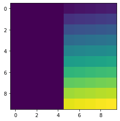
For example, we can update the values on the left part of this array to be equal to 1.

arr = np.arange(100).reshape(10,10)
arr[:, :5] = 1

plt.imshow(arr)

<matplotlib.image.AxesImage at 0x7f33274d7198>

The indexes in the square brackets of arr[:, :5] can be broken down like this:

[ 1st dimension start : 1st dimension end, 2nd dimension start : 2nd dimension end ]

Dimensions are separated by the comma ,. Our first dimension is the vertical axis, and the second dimension is the horizontal axis. Their spans are marked by the colon :. Therefore:

[ Vertical start : Vertical end, Horizontal start : Horizontal end ]

If there are no indexes entered, then the array will take all values. This means [:, :5] gives:

[ Vertical start : Vertical end, Horizontal start : Horizontal start + 5 ]

Therefore the array index selected the first 5 pixels along the width, at all vertical values.

Now let’s see what that looks like on an actual image.

Tip: Ensure you uploaded the file Guinea_Bissau.JPG to your Training folder along with the tutorial notebook. We will be using this file in the next few steps and exercises.

We can use the pyplot library to load an image using the matplotlib function imread. imread reads in an image file as a 3-dimensional numpy array. This makes it easy to manipulate the array.

By convention, the first dimension corresponds to the vertical axis, the second to the horizontal axis and the third are the Red, Green and Blue channels of the image. Red-green-blue channels conventionally take on values from 0 to 255.

im = np.copy(plt.imread('Guinea_Bissau.JPG'))

# This file path (red text) indicates 'Guinea_Bissau.JPG' is in the
# same folder as the tutorial notebook. If you have moved or
# renamed the file, the file path must be edited to match.

im.shape

(590, 602, 3)

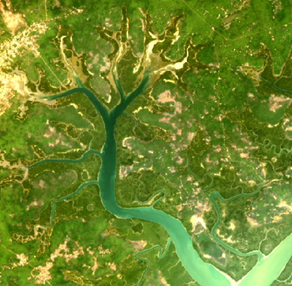
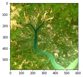
Guinea_Bissau.JPG is an image of Rio Baboque in Guinea-Bissau in 2018. It has been generated from Landsat 8 satellite data.

The results of the above cell show that the image is 590 pixels tall, 602 pixels wide, and has 3 channels. The three channels are red, green, and blue (in that order).

Let’s display this image using the pyplot imshow function.

plt.imshow(im)

<matplotlib.image.AxesImage at 0x7f33273bb400>

Exercises

3.1 Let’s use the indexing functionality of numpy to select a portion of this image. Select the top-right corner of this image with shape (200,200).

Hint: Remember there are three dimensions in this image. Colons separate spans, and commas separate dimensions.

# We already defined im above, but if you have not,
# you can un-comment and run the next line

# im = np.copy(plt.imread('Guinea_Bissau.JPG'))

# Fill in the question marks with the correct indexes

topright = im[?,?,?]

# Plot your result using imshow

plt.imshow(topright)

If you have selected the correct corner, there should be not much water in it!

3.2 Let’s have a look at one of the pixels in this image. We choose the top-left corner with position (0,0) and show the values of its RGB channels.

# Run this cell to see the colour channel values

im[0,0]

The first value corresponds to the red component, the second to the green and the third to the blue. uint8 can contain values in the range [0-255] so the pixel has a lot of red, some green, and not much blue. This pixel is a orange-yellow sandy colour.

Now let’s modify the image.

What happens if we set all the values representing the blue channel to the maximum value?

# Run this cell to set all blue channel values to 255
# We first make a copy to avoid modifying the original image

im2 = np.copy(im)

im2[:,:,2] = 255

plt.imshow(im2)

The index notation [:,:,2] is selecting pixels at all heights and all widths, but only the 3rd colour channel.

Can you modify the above code cell to set all red values to the maximum value of 255?

Conclusion

We have successfully practised indexing numpy arrays and plotting those arrays using matplotlib. We can now also read a file into Python using pyplot.imread. The next lesson covers data cleaning and masking.