Python basics 4: Cleaning data

This tutorial explores further concepts in Numpy such as categorical data, advanced indexing and dealing with Not-a-Number (NaN) data.

Follow the instructions below to download the tutorial and open it in the Sandbox.

Download the tutorial notebook

Download the Python basics 4 tutorial notebook

To view this notebook on the Sandbox, you will need to first download it to your computer, then upload it to the Sandbox. Ensure you have followed the set-up prerequisities listed in Python basics 1: Jupyter, and then follow these instructions:

1. Download the notebook by clicking the link above.

2. On the Sandbox, open the Training folder.

3. Click the Upload Files button as shown below.

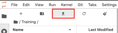
4. Select the downloaded notebook using the file browser. Click OK.

5. The solution notebook will appear in the Training folder. Double-click to open it.

You can now use the tutorial notebook as an interactive version of this webpage.

Note

The tutorial notebook should look like the text and code below. However, the tutorial notebook outputs are blank (i.e. no results showing after code cells). Follow the instructions in the notebook to run the cells in the tutorial notebook. Refer to this page to check your outputs look similar.

Numpy dictionaries and categorical data

We will introduce a numpy structure called a dictionary. This will be useful for the next lesson on xarray.

A dictionary represents a mapping between keys and values. The keys and values are Python objects of any type. We declare a dictionary using curly braces {}. Inside we specify the key then its associated value, with the keys and values separated by a colon :. Commas , are used to separate elements in the dictionary.

dictionary_name = {key1: value1, key2: value2, key3: value3}

For example:

d = {1: 'one',
     2: 'two',
     3: 'apple'}

In the above dictionary d, we have three keys 1, 2, 3, and their respective values 'one', 'two' and 'apple'.

We can look up elements in a dictionary using the [ key_name ] to address the value stored under a key. The syntax looks like:

dictionary_name[key_name]

In our example dictionary d above, we can call upon the value associated with the key name 1 like so:

d[1]

print(d[1], " + ", d[2], " = ", d[3])

Elements in a dictionary can be modified or new elements added by using the dictionary_name[key_name] = value syntax.

d[3] = 'three'
d[4] = 'four'

print(d[1], " + ", d[2], " = ", d[3])

Again, the dictionary name, key name, and value must be specified.

Dictionaries are useful for data analysis (including satellite data analysis) because they make it easy to assign categorical values to our dataset. Remote sensing can be used to create classification products that use categorical values. These products do not contain continuous values. They use discrete values to represent different classes individual pixels can belong to.

As an example, the following cells simulate a very simple image containing three different land cover types. Value 1 represents area covered with grass, 2 croplands and 3 city.

First, we import the libraries we want to use.

%matplotlib inline

import numpy as np
from matplotlib import pyplot as plt
from matplotlib import colors

We will now create a 2-dimensional 100 pixel x 100 pixel numpy array where every value is 1. This is done using the numpy.ones function. Then, we use array indexing to assign part of the area to have the value 2, and another part to have the value 3.

# grass = 1
area = np.ones((100,100))

# crops = 2
area[10:60,20:50] = 2

# city = 3
area[70:90,60:80] = 3

area.shape, area.dtype

((100, 100), dtype('float64'))

area

array([[1., 1., 1., ..., 1., 1., 1.],
       [1., 1., 1., ..., 1., 1., 1.],
       [1., 1., 1., ..., 1., 1., 1.],
       ...,
       [1., 1., 1., ..., 1., 1., 1.],
       [1., 1., 1., ..., 1., 1., 1.],
       [1., 1., 1., ..., 1., 1., 1.]])

We now have a matrix filled with 1s, 2s and 3s. At this point, there is no association between the numbers and the different types of ground cover.

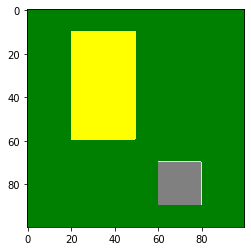
If we want to show what the area looks like according to the grass/crops/city designation, we might want to give each of the classifications a colour.

# We map the values to colours
index = {1: 'green', 2: 'yellow', 3: 'grey'}

# Create a discrete colour map
cmap = colors.ListedColormap(index.values())

# Plot
plt.imshow(area, cmap=cmap)

<matplotlib.image.AxesImage at 0x7fe7b5487f98>

In the case above, every pixel had a value of either 1, 2 or 3. What happens if our dataset is incomplete and there is no data in some places?

This is a common problem in real-life datasets. Real datasets can be incomplete and may be missing data at certain times or places. To deal with this, we use the special value known as NaN, which stands for Not a Number.

NaNs are designated by the numpy np.nan function.

arr = np.array([1,2,3,4,5,np.nan,7,8,9], dtype=np.float32)

arr

array([ 1.,  2.,  3.,  4.,  5., nan,  7.,  8.,  9.], dtype=float32)

To compute statistics on arrays containing NaN values, numpy has special versions of common functions such as mean, standard deviation std, and sum that ignore the NaN values. For example, the next cell shows the difference between using the usual mean function and the nanmean function.

The mean function cannot handle NaN values so it will return nan. The nanmean function does not include NaN values in the calculation, and therefore returns a number value.

print(np.mean(arr))

print(np.nanmean(arr))

nan
4.875

Note that NaN is generally not used as a key in dictionary key-value entries because there are different ways of expressing NaN in Python and they are not always equivalent. However, it is still possible to visualise data with NaNs; there will be gaps in the image where there is no data.

Exercises

4.1 The harvesting season has arrived and our cropping lands have changed colour to brown. Can you:

4.1.1 Modify the yellow area to contain the new value 4?

4.1.2 Add a new entry to the index dictionary mapping number 4 to the value brown.

4.1.3 Plot the area.

# 4.1.1 Modify the yellow area to hold the value 4

# 4.1.2 Add a new key-value pair to index that maps 4 to 'brown'

# 4.1.3 Copy the cmap definition and re-run it to add the new colour

# Plot the area

Hint: If you want to plot the new area, you have to redefine cmap so the new value is assigned a colour in the colour map. Copy and paste the cmap = ... line from the original plot.

4.2 Set area[20:40, 80:95] = np.nan. Plot the area now.

# Set the nan area

# Plot the entire area

4.3 Find the median of the area array from 4.2 using np.nanmedian. Does this match your visual interpretation? How does this compare to using np.median?

# Use np.nanmedian to find the median of the area

Conclusion

Two key Python capabilities have been introduced in this section. We can organise our data using the dictionary syntax, and understand incomplete datasets that may use NaN values to show blanks. The next lesson provides a guide to xarray, a Python package that builds on these concepts to make multi-dimensional data easier to load and use.