Python basics 5: Xarray¶

This tutorial introduces xarray (pronounced ex-array), a Python library for working with labeled multi-dimensional arrays. It is widely used to handle Earth observation data, which often involves multiple dimensions — for instance, longitude, latitude, time, and channels/bands. It can also display metadata such as the dataset Coordinate Reference System (CRS).

Accessing data held in an xarray.DataArray or xarray.Dataset is very similar to calling values from dictionaries.

Note: This tutorial is about using xarray. An introduction to remote sensing datasets and more information on Earth observation products used on the Digital Earth Africa platform can be found in Session 2: Digital Earth Africa products.

Follow the instructions below to download the tutorial and open it in the Sandbox.

Download the tutorial notebook¶

Download the Python basics 5 tutorial notebook

Download the exercise NetCDF file

To view this notebook on the Sandbox, you will need to first download the notebook and the NetCDF file to your computer, then upload both of them to the Sandbox. Ensure you have followed the set-up prerequisities listed in Python basics 1: Jupyter, and then follow these instructions:

Download the notebook by clicking the first link above. Download the image by clicking the second link above.
On the Sandbox, open the Training folder.
Click the Upload Files button as shown below.

Upload button.

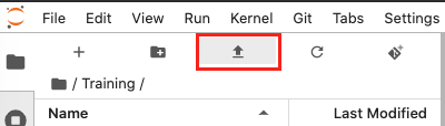
Select the downloaded notebook using the file browser. Click OK.
Repeat to upload the NetCDF (.nc) file to the Training folder. It may take a while for the upload to complete.
Both files will appear in the Training folder. Double-click the tutorial notebook to open it and begin the tutorial.

You can now use the tutorial notebook as an interactive version of this webpage.

Note

The tutorial notebook should look like the text and code below. However, the tutorial notebook outputs are blank (i.e. no results showing after code cells). Follow the instructions in the notebook to run the cells in the tutorial notebook. Refer to this page to check your outputs look similar.

Introduction to xarray¶

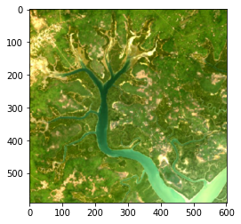
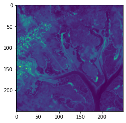
Xarray makes datasets easier to interpret when performing data analysis. To demonstrate this, we can start by opening a NetCDF file ( file suffix .nc) of the area of Guinea-Bissau we used in the previous matplotlib lesson.

Recap: In that lesson, we plotted the .JPG version of the image using imread and imshow.

[1]:

# Review of Python basics lesson 3: matplotlib

%matplotlib inline

import numpy as np
from matplotlib import pyplot as plt

im = np.copy(plt.imread('Guinea_Bissau.JPG'))
plt.imshow(im)

[1]:

<matplotlib.image.AxesImage at 0x7f6fc79feba8>

../_images/python_basics_05_xarray_9_1.png

Using xarray, we will now read in a .nc file of the area. .nc NetCDF files are a filetype used for storing scientific array-oriented data. Remembering that image data is an array, this makes both formats almost equivalent.

We could also load the .JPG as a dataset using xarray, but the NetCDF file contains more metadata so it will be easier to interpret.

As usual, we will first import the xarray package.

[2]:

# Import the xarray package as xr

import xarray as xr

[3]:

# Use xarray to open the data file

guinea_bissau = xr.open_dataset('guinea_bissau.nc')

[4]:

# Inspect the xarray.DataSet by
# typing its name

guinea_bissau

Let’s inspect the data. This image (our dataset) has a height y of 501 pixels and a width x of 500 pixels. It has 3 variables, which correspond to the red, green, and blue bands needed to plot a colour image. Each of these bands has a value at each of the pixels, so we have a total of 751500 values (the result of 501 x 500 x 3). Each of the x and y values are associated with a longitude and latitude and their values are stored under the Coordinates section.

The xarray.DataSet uses numpy arrays in the backend. What we see above is functionally similar to a bunch of numpy arrays holding the image band measurements and the longitude/latitude coordinates, combined with a dictionary of key-value pairs that defines the Attributes such as CRS and resolution (res). That sounds more complicated, doesn’t it? Accessing the data through xarray avoids the complications of managing uncorrelated numpy arrays by themselves.

Xarray dataset breakdown

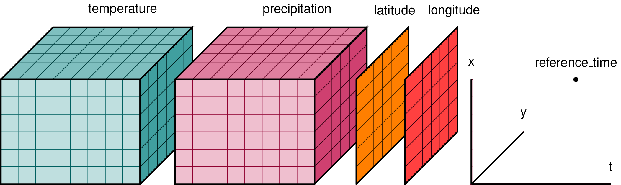
A visualisation of an xarray.Dataset. The coordinates are each a single dimension; latitude, longitude and time. Each variable (in this case temperature and precipitation) holds one value at each of the three coordinate dimensions.

An xarray.Dataset can be seen as a dictionary structurefor packing up the data, dimensions and attributes all linked together.

As in the NetCDF we loaded above, Digital Earth Africa follows the convention of storing spectral bands as separate variables, with each one as 3-dimensional cubes containing the temporal dimension.

To access a single variable we can use the same format as if it were a Python dictionary.

var = dataset_name['variable_name']

Alternatively, we can use the . notation.

var = dataset_name.variable_name

A single variable pulled from an xarray.Dataset is known as an xarray.DataArray. In the visualisation image above, the example xarray.Dataset is formed out of two xarray.DataArrays — one each for temperature and precipitation.

Note: Variable names are often strings (enclosed in quotation marks). This is true of most Digital Earth Africa datasets, where variables such as satellite bands have names such as 'red', 'green', 'nir'. Do not forget the quotation marks in first call method above, or the data will not load.

The dataset we loaded only has 1 timestep. We will now pull just the 'red' variable data from our guinea_bissau xarray.Dataset, and then plot it.

[5]:

guinea_bissau['red']

# This is equivalent to
# guinea_bissau.red
# Try it!

[6]:

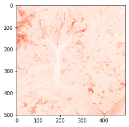
# Plot using imshow

plt.imshow(guinea_bissau['red'], cmap='Reds')

[6]:

<matplotlib.image.AxesImage at 0x7f6fb0b77400>

../_images/python_basics_05_xarray_22_1.png

Note: cmap stands for ‘colour map’. What happens if you remove this argument? plt.imshow will then plot all the red data values in the default colour scheme, which is a purple-to-yellow sequential colour map known as viridis. This is because matplotlib does not know the variable name red is associated with the colour red — it is just a name. You can find out more about matplotlib colourmaps through this matplotlib tutorial.

We stated above that xarray uses numpy arrays in the backend. You can access these numpy arrays by adding .values after a DataArray name. In the example below, guinea_bissau.red is the DataArray name.

[7]:

guinea_bissau.red.values

[7]:

array([[1007., 1007., 1069., ...,  489.,  476.,  422.],
       [ 988.,  991., 1048., ...,  456.,  459.,  444.],
       [ 976., 1023., 1062., ...,  453.,  454.,  448.],
       ...,
       [ 518.,  518.,  546., ...,  551.,  577.,  553.],
       [ 517.,  527.,  523., ...,  530.,  572.,  570.],
       [ 502.,  490.,  473., ...,  545.,  576.,  580.]])

It is possible to index xarray.DataArrays by position using the numpy [:,:] syntax we introduced in previous lessons, without converting to numpy arrays. However, we can also use the xarray syntaxes, which explictly label coordinates instead of relying on knowing the order of dimensions.

Each method is demonstrated below.

[:,:]: numpy syntax — requires knowing order of dimensions and positional indexes
isel(coordinate_name = coordinate_index): index selection — xarray syntax for selecting data based on its positional index (similar to numpy)
sel(coordinate_name = coordinate_value): value selection — xarray syntax for selecting data based on its value in that dimension

For example, we can call out the value of green in the top leftmost pixel of the image dataset.

[8]:

# Using numpy syntax

guinea_bissau.green[0,0]

In this case our positional indexes for x and y are the same, but it is important to note y is the first dimension, and x is the second. This is not immediately obvious and can cause confusion. For this reason, it is recommended to use one of the xarray syntaxes shown below. They explicitly call on the dimension names.

[9]:

# Using index selection, isel()

guinea_bissau.green.isel(y=0, x=0)

As before, the measurement for green in the top leftmost pixel is 730. In this example, the values of x and y are latitude and longitude values, but their positional indexes are 0.

We can call out the value by using the index, as shown below.

Note: The CRS we are using has units of metres. This means the x and y values are measured in metres.

[10]:

# The value of x at the pixel located at index (0,0)

guinea_bissau.green.x[0].values

[10]:

array(388020.)

[11]:

# The value of y at the pixel located at index (0,0)

guinea_bissau.green.y[0].values

[11]:

array(1338000.)

The intepretation of the cell above is:

Output the value of y in the 1st position of the green variable from the dataset called guineau_bissau.

We see the first element (index of 0) in x has a value of 388020 metres, and the first value of y is 1338000 metres.

How about the second method, sel()? This method was not available in the numpy arrays we used in previous lessons, and is one of the strengths of xarray as you can use the value of the dimension without knowing its positional index.

If we are given (y, x) = (1338000, 388020), we can find the green measurement at that point using sel().

[12]:

guinea_bissau.green.sel(y=1338000, x=388020)

Finally, we can select ranges of DataArrays with the xarray syntaxes using slice. The three cells below all extract the same extent from the guinea_bissau.green DataArray.

The xarray syntaxes for ranges using slice are:

dataarray_name.isel(dimension_name = slice(index_start, index_end))

dataarray_name.sel(dimension_name = slice(value_start, value_end))

As before, it is easier to call upon the dimensions by name rather than using the implicit numpy square bracket syntax, although it still works.

[13]:

# Numpy syntax - dimensions are not named
# Valid but not recommended

guinea_bissau.green[:250, :250]

[14]:

# Index selection slice

guinea_bissau.green.isel(x=slice(0,250), y=slice(0,250))

[15]:

# Value selection slice

guinea_bissau.green.sel(x=slice(388020,395500), y=slice(1338000,1330530))

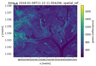
We can plot the selected area using matplotlib plt.imshow. We can also use the xarray .plot() function. Plotting is a good way to check the selection is showing the top left section of the image as expected.

The syntax of plt.imshow() is:

plt.imshow(data)

Therefore we copy the code into the brackets of plt.imshow().

[16]:

plt.imshow(guinea_bissau.green.sel(x=slice(388020,395500), y=slice(1338000,1330530)))

[16]:

<matplotlib.image.AxesImage at 0x7f6fb0af2470>

../_images/python_basics_05_xarray_43_1.png

Note: We did not specify a colourmap cmap so you can see it takes on the default colour scheme. Plotting true-colour (RGB) images is first introduced in Session 2: Loading data in the Sandbox.

The syntax of the xarray plot function is:

data.plot()

Therefore we copy the code before we type .plot().

[17]:

guinea_bissau.green.sel(x=slice(388020,395500), y=slice(1338000,1330530)).plot()

[17]:

<matplotlib.collections.QuadMesh at 0x7f6fb0a0cba8>

../_images/python_basics_05_xarray_47_1.png

The advantage of using xarray’s .plot() is that it automatically shows the x and y axes using coordinate values, not their positional index.

Exercises¶

5.1 Can you access to the `crs` value in the attributes of the `guinea_bissau` `xarray.Dataset`?¶

Hint: You can call upon attributes in the same way you would select a variable or coordinate.

[ ]:

# Replace the ? with the attribute name

guinea_bissau.?

5.2 Select the region of the `blue` variable delimited by these coordinates:¶

latitude of range [1335000, 1329030]
longitude of range [389520, 395490]

Hint: Do we want to use sel() or isel()? Which coordinate is x and which is y?

5.3 Plot the selected region using `imshow`, then plot the region using `.plot()`.¶

[ ]:

# Plot using plt.imshow

[ ]:

# Plot using .plot()

Can you change the colour map to `'Blues'`?¶

Conclusion¶

Xarray is an important tool when dealing with Earth observation data in Python. Its flexible and intuitive interface allows multiple methods of selecting data and performing analysis.

Python basics 5: Xarray¶

Download the tutorial notebook¶

Introduction to xarray¶

Exercises¶

5.1 Can you access to the crs value in the attributes of the guinea_bissau xarray.Dataset?¶

5.2 Select the region of the blue variable delimited by these coordinates:¶

5.3 Plot the selected region using imshow, then plot the region using .plot().¶

Can you change the colour map to 'Blues'?¶

Conclusion¶

5.1 Can you access to the `crs` value in the attributes of the `guinea_bissau` `xarray.Dataset`?¶

5.2 Select the region of the `blue` variable delimited by these coordinates:¶

5.3 Plot the selected region using `imshow`, then plot the region using `.plot()`.¶

Can you change the colour map to `'Blues'`?¶