Python basics 1: Jupyter

The first lesson of the Python basics session is on performing basic Python commands in a Jupyter Notebook. We will be using a prepared tutorial notebook to guide you through the steps.

Set-up prerequisites

The Python basics interactive tutorials use the Digital Earth Africa Sandbox platform. This requires a Digital Earth Africa Sandbox account.

To set up the learning environment, please complete all sections in Session 1: Introduction before starting this Python basics module.

Then, follow the instructions below to download the tutorial and open it in the Sandbox.

Download the tutorial notebook

Download the Python basics 1 tutorial notebook

To view this notebook on the Sandbox, you will need to first download it to your computer, then upload it to the Sandbox.

Note

Ensure you have created a Training folder in the Sandbox as instructed in Session 1: Running a Notebook.

Once you have created a Training folder, follow these instructions:

1. Download the notebook by clicking the link above.

2. On the Sandbox, open the Training folder.

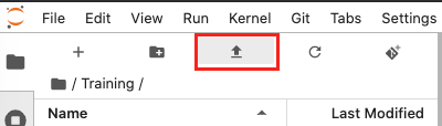
3. Click the Upload Files button as shown below.

4. Select the downloaded notebook using the file browser. Click OK.

5. The solution notebook will appear in the Training folder. Double-click to open it.

You can now use the tutorial notebook as an interactive version of this webpage.

Note

The tutorial notebook should look like the text and code below. However, the tutorial notebook outputs are blank (i.e. no results showing after code cells). Follow the instructions in the notebook to run the cells in the tutorial notebook. Refer to this page to check your outputs look similar.

Recap: Jupyter Notebooks

First, we will review the Python commands introduced in Session 1. This lesson provides more examples and additional detail to the explanations.

A Jupyter notebook is an interactive environment where you can combine text with with Python code that you can modify and execute. The gray cell below contains Python code that you can run. Place the cursor on the Run icon |►| in the menu at the top of the notebook to execute the code inside.

Tip: Use the shortcut Shift+Enter for running the active cell (where your cursor is). It is a convenient trick that saves you from having to click on the Run icon each time.

Select and run the grey code cell below.

print("Welcome to the Digital Earth Africa Sandbox!")

You’ll see that once the code has executed, any output generated by your code will show up just below the cell.

print("3,2,1")

# # Use the hash symbol to comment lines of your code. This does not get executed.
# # Use comments to make notes about what your code is doing.

print("this is fun!")

We can do mathematical computation using Python. Below, we have assigned the sum to a variable. We have chosen to name this variable result.

# Set this sum as a variable called result
result = 999 + 1

# The output of result is displayed once the computation is completed
result

The [ ]: symbol to the left of each code cell describes the state of the cell:

• [ ]: means that the cell has not been run yet.

• [*]: means that the cell is currently running.

• [1]: means that the cell has finished running and was the first cell run.

Sometimes, the code that you run in a cell takes a while to compute because it is loading a large dataset or performing complex computations. You’ll notice the number that appears next to the cell. Before the cell is run you’ll see the symbol [ ] meaning that cell has not been executed yet. While a cell is running it shows the [*] symbol and once it has completed running you’ll see a number representing the number of cells being run, for example [4]. This allows you to keep track of the cells that have been run and their relative order.

Note: To check whether a cell is currently executing in a Jupyter notebook, inspect the small circle in the top-right of the window. The circle will turn black (“Kernel busy”) when the cell is running, and return to white (“Kernel idle”) when the process is complete.

Consider this Python program. Here, we have decided to call our variable a.

a = 1
print(a)
a = a + 1
print(a)

We can break down this program and execute each line using separate cells.

Note: Python is case sensitive. The variable a is not the same as A.

a = 1

print(a)

a = a + 1

print(a)

If you run again the first a cell you’ll see that it returns 2, the updated value. This is called ‘global state’, and means that once a variable is declared it is accessible anywhere in the notebook, even in cells above where it has been declared. This is different to traditional programs which execute sequentially line by line from the top to the bottom. This can be confusing in the beginning, but keep an eye on the number in the brackets [ ] to see cell execution order.

This also means you can modify all the code in the cells and run them as many times as you want in any order. You can jump back and forth to update variables or re-run analysis.

Exercises

1.1 Fill the asterisk line with your name and run the cell.

# Fill the ****** space with your name and run the cell.

message = "My name is ******"

message

1.2 You can add new cells to insert new code at any point in a notebook. Click on the + icon in the top menu to add a new cell below the current one. Add a new cell below the next cell, and use it to print the value of variable a.

a = 365*24

# Add a new cell just below this one. Use it to print the value of variable `a`

Question: Now what happens if you scroll back up the notebook and execute a different cell containing print(a)?

Conclusion

Well done on finishing the recap lesson on Jupyter Notebooks. You are now ready to learn about Numpy! Click Next to continue.